1. Rainfall-Runoff Models
BEGIN
Rainfall-Runoff Models

2. Excess Precipitation or Runoff Volume Models
May be:
Physically Based
Empirical
Descriptive
Conceptual
Generally Lumped
Etc……
May not only estimate excess precipitation – hence, we will refer to them as rainfall-runoff models…..

3. The Basic Process…. Focus on Excess Precipitation Excess Precip. Model
Necessary for a single basin
Focus on Excess Precipitation
Excess Precip. Model
Excess Precip.
Basin “Routing” UHG Methods
Runoff Hydrograph
Excess Precip.
Stream and/or Reservoir “Routing”
Downstream Hydrograph
Runoff Hydrograph

4. Goal of Rainfall-Runoff Models
The fate of the falling precipitation is:
…modeled in order to account for the destiny of the precipitation that falls and the potential of the precipitation to affect the the runoff hydrograph.
… losses include interception, evapotranspiration, storage, infiltration, percolation, and finally - runoff.
Let’s look at the fate of the precipitation…..

5. Interception
First, the falling precipitation may be intercepted by the vegetation in an area.
It is typically either distributed as runoff or evaporated back to the atmosphere.
The leafy matter may also be a form of interception.

6. Canopy…(or lack of)

7. Leafy Matter also intercepts...
Very thick ground litter layers can hold as much as 0.5 inches!

8. Interception…the point
The point of the interception is that the precipitation is temporarily stored before the next process begins.
The intercepted/stored precipitation may not reach the ground to contribute to runoff.
Interception may be referred to as an abstraction and is accounted for as initial abstraction in some models.
This is also true for snowfall which may sublimate and leave the watershed!

9. Infiltration
Precipitation reaching the ground may infiltrate.
This is the process of moving from the atmosphere into the soil.
Infiltration may be regarded as either a rate or a total. For example: the soil can infiltrate 1.2 inches/hour. Alternatively, we could say the soil has a total infiltration capacity of 3 inches.
Note that in both cases the units are Length or length per time!

10. Infiltration, cont
Infiltration is nearly impossible to measure directly - as we would disturb the sample in doing so.
We can infer infiltration in a variety of ways (to be discussed at a later point).
The exact point at which the atmosphere ends and the soil beings is very difficult to define and generally we are not concerned with this fine detail!
In other words, we mostly want to know how much of the precipitation actually enters the soil.

11. Percolation.....
Once the water infiltrates into the ground, the downward movement of water through the soil profile may begin.

12. Percolation.....
The percolating water may move as a saturated front - under the influence of gravity…

13. Percolation.....
Or, it may move as unsaturated flow mostly due to capillary forces.

14. Percolation….the point
The vertical percolation of the water into various levels or zones allows for storage in the subsurface – these zones will be very important in the SAC-SMA model.
This stored subsurface water is held and released as either evaporation, transpiration, or as streamflow eventually reaching the watershed outlet.

15. Evaporation....
Is the movement of water from the liquid state to the vapor state - allowing transport to the atmosphere.
Occurs from any wet surface or open body of water.
Soil can have water evaporate from within, as can leafy matter, living leaves and plants, etc..
The water evaporates from a storage location....

16. Transpiration....
The process of water moving from the soil via the plants internal moisture supply system.
This is a type of evaporative process.
The water moves through the stomates, tiny openings in the leaves (mostly on the underside), that allow the passage of oxygen, carbon dioxide, water vapor, and other gases.

17. Evapotranspiration....
The terms transpiration and evaporation are often combined in the form :
EVAPOTRANSPIRATION

18. Storage....
Storage occurs at several “locations” in the hydrologic cycle and varies in both space and time - spatially and temporally.
Water can be stored in:
The unsaturated portion of the soil
The saturated portion (below the water table)
On the soil or surface - snow/snowpack, puddles, ponds, lakes, wetlands.
Rivers and stream channels - even though they are generally in motion!

19. Storage.... Water in storage can still be involved in a process.
i.e. :
Water in a puddle may be evaporating.....

20. The hydrologic cycle represented as a series of storage units & processes....- RO = P E T
Depression Storage
Surface runoff
Storm Flow
Is I > f?
yes
Channel Storage
Base Flow no
Channel runoff
Detention Storage
Is retention full?
yes
Surface runoff
Ground Water Storage no
Retention Storage
Vegetation Storage

21. Storage.... - = The thought process....... RO P T E RO Pno
yes
Base Flow
Is retention full?
Surface runoff
Storm Flow
Is I > f?
Channel Storage
Depression Storage
Ground Water Storage
Detention Storage
Retention Storage
Vegetation Storage
Is I > f?
yes
Surface runoff
Channel runoff

22. Storage.... Things to consider:
We looked at these as independent processes!
We looked at the processes as discrete time steps!
What were the initial conditions before the storm? What effects would initial conditions have?
These are the issues that a continuous rainfall-runoff model must consider……

23. The Units The units are very important…
Storage is a volume (L3) and flow is a volume per time (L3/T) ….
We often think of these volume units in terms of length only!
This implies a uniform depth or value throughout the watershed….

24. Examples of Length Units for Storage
The watershed can infiltrate 75mm of water – a length…
The lower zone of the soil can hold 60mm...
The initial abstraction for the watershed is 10mm
The reservoir can hold 2.5 inches of runoff…
These all imply uniformity over the watershed…

25. The Rainfall-Runoff Modeling Process
… simplistic methods such as a constant loss method may be used.
… A constant loss approach assumes that the soil can constantly infiltrate the same amount of precipitation throughout the storm event. The obvious weaknesses are the neglecting of spatial variability, temporal variability, and recovery potential.
Other methods include exponential decays (the infiltration rate decays exponentially), empirical methods, and physically based methods.
… There are also combinations of these methods.

26. Initial Abstractions
Initial Abstraction - It is generally assumed that the initial abstractions must be satisfied before any direct storm runoff may begin. The initial abstraction is often thought of as a lumped sum (depth). Viessman (1968) found that 0.1 inches was reasonable for small urban watersheds.
Would forested & rural watersheds be more or less?

27. Rural watersheds would probably have a higher initial abstraction.
The Soil Conservation Service (SCS) now the NRCS uses a percentage of the ultimate infiltration holding capacity of the soil - i.e. 20% of the maximum soil retention capacity.

28. Some Rainfall-Runoff Models
Phi-Index
Horton Equation
SCS Curve Number
SAC-SMA

29. Constant Infiltration Rate
A constant infiltration rate is the most simple of the methods. It is often referred to as a phi-index or f-index.
In some modeling situations it is used in a conservative mode.
The saturated soil conductivity may be used for the infiltration rate.
The obvious weakness is the inability to model changes in infiltration rate.
The phi-index may also be estimated from individual storm events by looking at the runoff hydrograph.

30. Hydrograph Breakdown

31. Hydrograph Breakdown

32. Derive phi-index sample watershed = 450 mi2

33. Separation of Baseflow
... generally accepted that the inflection point on the recession limb of a hydrograph is the result of a change in the controlling physical processes of the excess precipitation flowing to the basin outlet.
… In this example, baseflow is considered to be a straight line connecting that point at which the hydrograph begins to rise rapidly and the inflection point on the recession side of the hydrograph.
… the inflection point may be found by plotting the hydrograph in semi-log fashion with flow being plotted on the log scale and noting the time at which the recession side fits a straight line.

34. Semi-log Plot

35. Hydrograph & Baseflow

36. Separate Baseflow

37. Sample Calculations
In the present example (hourly time step), the flows are summed and then multiplied by 3600 seconds to determine the volume of runoff in cubic feet. If desired, this value may then be converted to acre-feet by dividing by 43,560 square feet per acre.
The depth of direct runoff in feet is found by dividing the total volume of excess precipitation (now in acre-feet) by the watershed area (450 mi2 converted to 288,000 acres).
In this example, the volume of excess precipitation or direct runoff for storm #1 was determined to be 39,692 acre-feet.
The depth of direct runoff is found to be feet after dividing by the watershed area of 288,000 acres.
Finally, the depth of direct runoff in inches is x 12 = 1.65 inches.

38. Summing Flows
Continuous process represented with discrete time steps

39. Estimating Excess Precip.
0.8
1.65 inches of excess precipitation
0.7
0.6
0.5
Uniform loss rate of
Precipitation (inches)
0.2 inches per hour.
0.4
0.3
0.2
0.1 1 2 3 4 5 6 7 8 9 10 11 12 13 14 15 16 17 18 19
Time (hrs.)

40. Phi-Index Summary
The phi-index for this storm was 0.2 inches per hour.
This is a uniform loss rate.
If the precipitation stops for a time period, the infiltration will still be 0.2 inches per hour when the precipitation starts again.
Regardless of this weakness, this is still very powerful information to have regarding the response of a watershed.

41. Exponential Decay - Horton
This is purely a mathematical function - of the following form: fo
fi = infiltration capacity at time, t
fc = final infiltration capacity
fo = initial infiltration capacity fc

42. Horton
Effect of fo or fc

43. Horton
Effect of K

44. Horton
Assumes that precipitation supply is greater than infiltration rate. 2 1

45. Horton
There are now 2 parameters to estimate or calibrate for a watershed!!
fo & k

46. Horton – Issues with Continuous Simulation
Again, if it stops raining how does the soil recover in a Horton model?
i.e.
Stopped raining for a short period – how does the soil recover?

47. SCS Curve Number
Soil Conservation Service is an empirical method of estimating EXCESS PRECIPITATION
We can imply that precipitation minus excess precipitation = infiltration/retention :
P - Pe = F

48. SCS (NRCS) Runoff Curve Number
The basic relationships used to develop the curve number runoff prediction technique are described here as background for subsequent discussion. The technique originates with the assumption that the following relationship describes the water balance of a storm event.
where F is the actual retention on the watershed, Q is the actual direct storm runoff, S is the potential maximum retention, and P is the potential maximum runoff

49. Modifications
Pe = P - Ia
Effective precipitation equals total precipitation minus initial abstraction…
We will use effective precipitation in place of precipitation…

50. More Modifications
At this point in the development, SCS redefines S to be the potential maximum retention
SCS also defines Ia in terms of S as : Ia = 0.2S
A little substituting gives the familiar SCS rainfall-runoff equation:

51. Estimating “S” CN ranges from 1 to 100 (not really!)
The difficult part of applying this method to a watershed is the estimation of the watershed’s potential maximum retention, S.
SCS developed the concept of the dimensionless curve number, CN, to aid in the estimation of S.
CN is related to S as follows :
CN ranges from 1 to 100 (not really!)

52. Determine CN
The Soil Conservation Service has classified over 8,500 soil series into four hydrologic groups according to their infiltration characteristics, and the proper group is determined for the soil series found.
The hydrologic groups have been designated as A, B, C, and D.
Group A is composed of soils considered to have a low runoff potential. These soils have a high infiltration rate even when thoroughly wetted.
Group B soils have a moderate infiltration rate when thoroughly wetted,
while group C soils are those which have slow infiltration rates when thoroughly wetted.
Group D soils are those which are considered to have a high potential for runoff, since they have very slow infiltration rates when thoroughly wetted (SCS, 1972).

53. Determine CN, cont….
Once the hydrologic soil group has been determined, the curve number of the site is determined by cross-referencing land use and hydrologic condition to the soil group - SAMPLE
Land use and treatment Hydrologic soil group
or Hydrologic
practice condition A B C D
Fallow
Straight row
Row Crops
Straight row Poor
Straight row Good
Contoured Poor

54. 5-day antecedent rainfall, inches
Initial Conditions
5-day antecedent rainfall, inches
Antecedent moisture
Dormant Season Growing Season
I Less than 0.5 Less than 1.4
II 0.5 to to 2.1
III Over Over 2.1

55. Adjust CN’s

56. Sample Application The curve number is assumed to be 70.
The cumulative runoff (c) is calculated from the cumulative precipitation (b), using equation (4).
The potential maximum storage, S, is calculated to be S = (1000/70) - 10 = inches.
Using 20% as the initial abstraction percentage yields 0.2 x = inches and will require that at least inches of precipitation must accrue before runoff may begin.

57. Computations

58. Problems
The initial abstraction (Ia) consists of interception, depression storage, and infiltration that occurs prior to runoff.
It is not easy to estimate the initial abstraction for a particular storm event.
SCS felt that there should be a connection between Ia versus S, and they attempted to develop the relationship by plotting Ia versus S for a large number of events on small experimental watersheds. - Quite a SCATTER - not very successful.

59. These rainfall-runoff models have varied in complexity – but would have difficulty in modeling a continuous event, as they all lack the ability to allow the soil zones to “recover” when the precipitation stops….. This leads us to model systems that are intended for continuous simulation with “updating” abilities.

60. SAC-SMA
… The Sacramento Soil Moisture Accounting Model (SAC-SMA) is a conceptual model of soil moisture accounting that uses empiricism and lumped coefficients to attempt to mimic the physical constraints of water movement in a natural system.

61. Sacramento Soil Moisture Accounting Model

62. Sacramento Model Structure
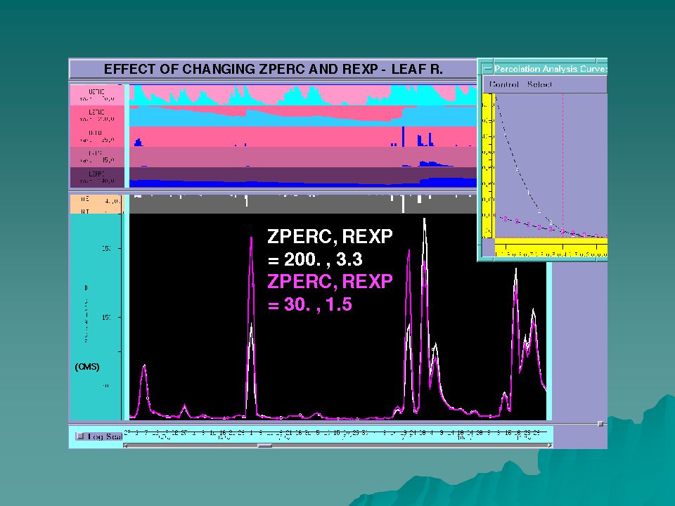
E T Demand
Impervious
Area
E T
Precipitation Input Px
Pervious Area
Impervious Area
Tension Water
UZTW Free Water
UZFW
Percolation
Zperc. Rexp
1-PFREE
PFREE
Free Water
Tension Water P S
LZTW LZFP LZFS
RSERV
Primary
Baseflow
Direct Runoff
Surface Runoff
Interflow
Supplemental
Base flow
Side
Subsurface Discharge
LZSK
LZPK
Upper Zone
Lower Zone
EXCESS
UZK
RIVA
PCTIM
ADIMP
Total Channel Inflow
Distribution Function
Streamflow
Total Baseflow

63. Hydrograph Decomposition
Supplemental Baseflow
Primary Baseflow
Interflow
Surface Runoff
Impervious and Direct Runoff
Discharge
Time

64. Sacramento Soil Moisture Components
Impervious and Direct Runoff
Surface Runoff
Interflow
Supplemental Baseflow
Primary Baseflow
SAC-SMA Model
Evaporation
Precipitation
Upper
Zone
Lower
Pervious
Impervious

65. Initial Soil-moisture Parameter Estimates By Hydrograph Analysis

66. Initial Soil-moisture Parameter Estimates By Hydrograph Analysis (continued)
LZSK - Supplemental baseflow recession (always > LZPK)
Flow that typically persists anywhere from 15 days to 3 or 4 months

67. Initial Soil Moisture Parameters Estimates by Hydrograph Analysis (continued)

68. Initial Soil Moisture Estimates by Hydrograph Analysis (continued)

69. Multiyear Statistical Output

70. Multiyear Statistical Output (continued)

96. Rainfall-Runoff Models
END
Rainfall-Runoff Models