1. Randomized / Hashing Algorithms
Shannon Quinn
(with thanks to William Cohen of Carnegie Mellon University, and J. Leskovec, A. Rajaraman, and J. Ullman of Stanford University)

2. Next Wednesday’s lecture
Outline
Bloom filters
Locality-sensitive hashing
Stochastic gradient descent
Stochastic SVD
Already covered
Next Wednesday’s lecture

3. Hash Trick - Insights Save memory: don’t store hash keys
Allow collisions
even though it distorts your data some
Let the learner (downstream) take up the slack
Here’s another famous trick that exploits these insights….

4. Bloom filters Interface to a Bloom filter
BloomFilter(int maxSize, double p);
void bf.add(String s); // insert s
bool bd.contains(String s);
// If s was added return true;
// else with probability at least 1-p return false;
// else with probability at most p return true;
I.e., a noisy “set” where you can test membership (and that’s it)
note a hash table would do this in constant time and storage
the hash trick does this as well

5. One possible implementation
BloomFilter(int maxSize, double p) { set up an empty length-m array bits[]; } void bf.add(String s) { bits[hash(s) % m] = 1; bool bd.contains(String s) { return bits[hash(s) % m];

6. How well does this work?
m=1,000, x~=200, y~=0.18

7. How well does this work?
m=10,000, x~=1,000, y~=0.10

8. A better??? implementation
BloomFilter(int maxSize, double p) { set up an empty length-m array bits[]; } void bf.add(String s) { bits[hash1(s) % m] = 1; bits[hash2(s) % m] = 1; bool bd.contains(String s) { return bits[hash1(s) % m] && bits[hash2(s) % m];

9. How well does this work? m=1,000, x~=13,000, y~=0.01

10. Bloom filters An example application Finding items in “sharded” data
Easy if you know the sharding rule
Harder if you don’t (like Google n-grams)
Simple idea:
Build a BF of the contents of each shard
To look for key, load in the BF’s one by one, and search only the shards that probably contain key
Analysis: you won’t miss anything, you might look in some extra shards
You’ll hit O(1) extra shards if you set p=1/#shards

11. Bloom filters An example application
discarding rare features from a classifier
seldom hurts much, can speed up experiments
Scan through data once and check each w:
if bf1.contains(w):
if bf2.contains(w): bf3.add(w)
else bf2.add(w)
else bf1.add(w)
Now:
bf2.contains(w)  w appears >= 2x
bf3.contains(w)  w appears >= 3x
Then train, ignoring words not in bf3

12. Bloom filters p = k = Analysis (m bits, k hashers):
Assume hash(i,s) is a random function
Look at Pr(bit j is unset after n add’s):
… and Pr(collision):
…. fix m and n and minimize k:
p =
k =

13. Bloom filters p = Analysis:
Plug optimal k=m/n*ln(2) back into Pr(collision):
Now we can fix any two of p, n, m and solve for the 3rd:
E.g., the value for m in terms of n and p:
p =

14. Bloom filters: demo

15. Locality Sensitive Hashing (LSH)
Two main approaches
Random Projection
Minhashing

16. LSH: key ideas Goal: map feature vector x to bit vector bx
ensure that bx preserves “similarity”

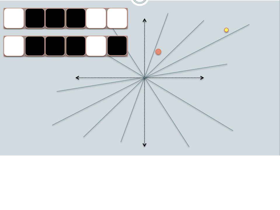
17. Random Projections

18. Random projections
To make those points “close” we need to project to a direction orthogonal to the line between them u + - -u 2γ

19. Random projections
Any other direction will keep the distant points distant. u + -
So if I pick a random r and r.x and r.x’ are closer than γ then probably x and x’ were close to start with. -u 2γ

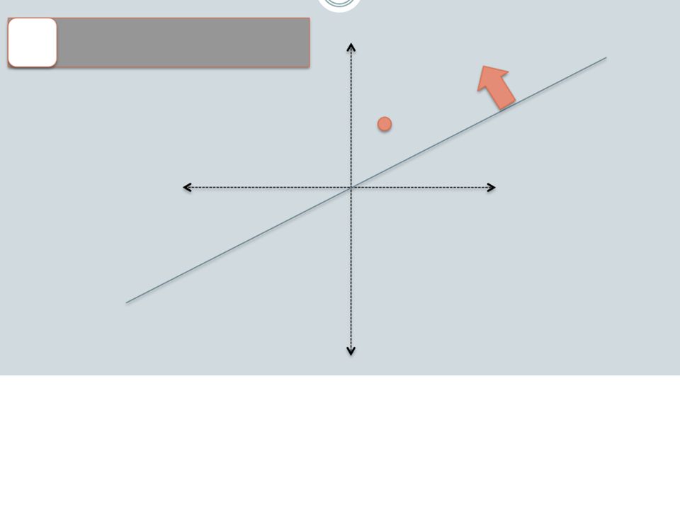
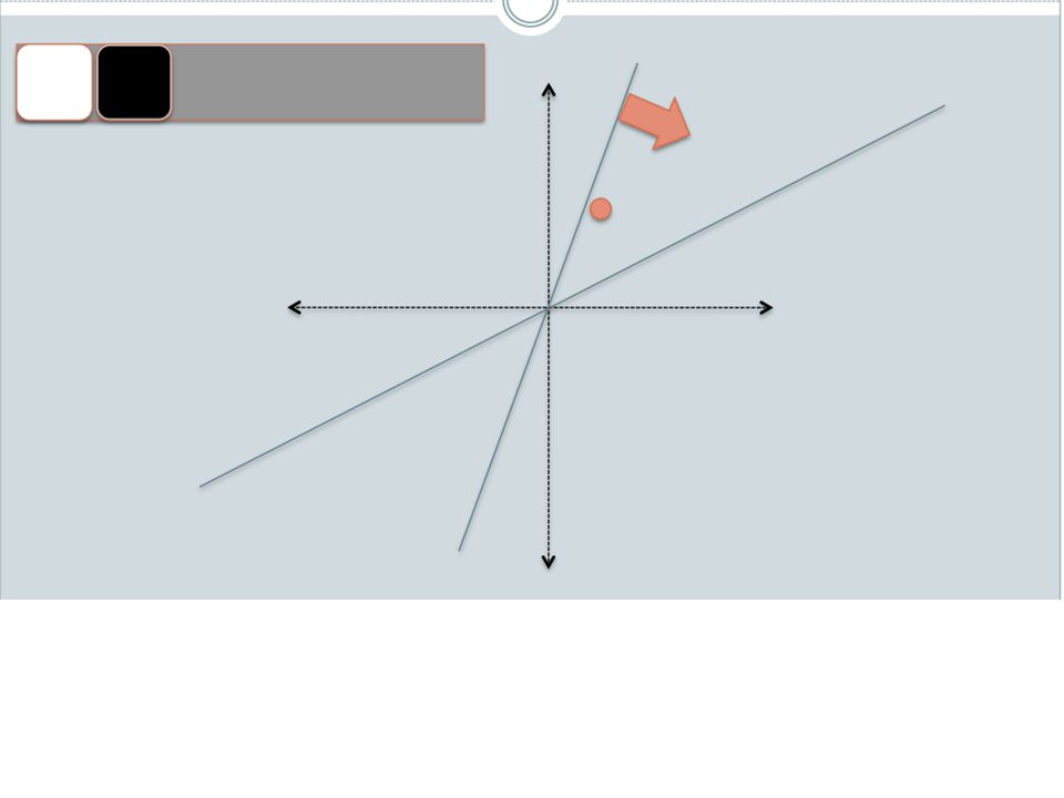
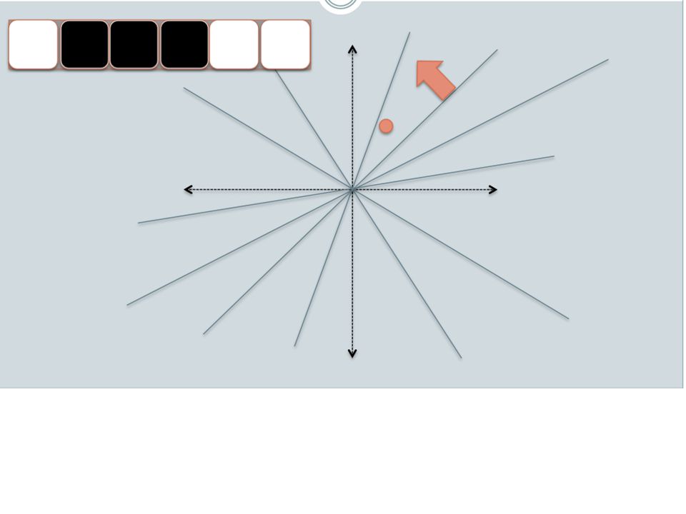
20. LSH: key ideas Goal: map feature vector x to bit vector bx
ensure that bx preserves “similarity”
Basic idea: use random projections of x
Repeat many times:
Pick a random hyperplane r
Compute the inner product of r with x
Record if x is “close to” r (r.x>=0)
the next bit in bx
Theory says that is x’ and x have small cosine distance then bx and bx’ will have small Hamming distance

21. LSH: key ideas Naïve algorithm: Initialization: Given an instance x
For i=1 to outputBits:
For each feature f:
Draw r(f,i) ~ Normal(0,1)
Given an instance x
LSH[i] =
sum(x[f]*r[i,f] for f with non-zero weight in x) > 0 ? 1 : 0
Return the bit-vector LSH
Problem:
the array of r’s is very large

29. Distance Measures Goal: Find near-neighbors in high-dim. space
We formally define “near neighbors” as points that are a “small distance” apart
For each application, we first need to define what “distance” means
Today: Jaccard distance/similarity
The Jaccard similarity of two sets is the size of their intersection divided by the size of their union: sim(C1, C2) = |C1C2|/|C1C2|
Jaccard distance: d(C1, C2) = 1 - |C1C2|/|C1C2|
3 in intersection
8 in union
Jaccard similarity= 3/8
Jaccard distance = 5/8
J. Leskovec, A. Rajaraman, J. Ullman: Mining of Massive Datasets,

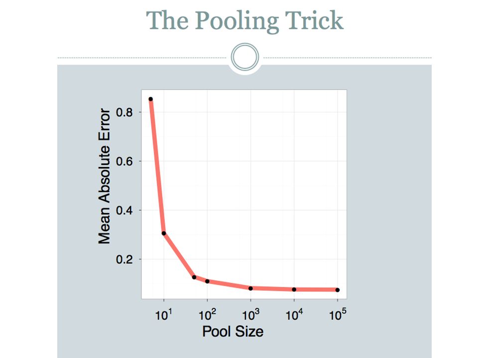
30. LSH: “pooling” (van Durme)
Better algorithm:
Initialization:
Create a pool:
Pick a random seed s
For i=1 to poolSize:
Draw pool[i] ~ Normal(0,1)
For i=1 to outputBits:
Devise a random hash function hash(i,f):
E.g.: hash(i,f) = hashcode(f) XOR randomBitString[i]
Given an instance x
LSH[i] = sum(
x[f] * pool[hash(i,f) % poolSize] for f in x) > 0 ? 1 : 0
Return the bit-vector LSH

32. LSH: key ideas: pooling
Advantages:
with pooling, this is a compact re-encoding of the data
you don’t need to store the r’s, just the pool
leads to very fast nearest neighbor method
just look at other items with bx’=bx
also very fast nearest-neighbor methods for Hamming distance
similarly, leads to very fast clustering
cluster = all things with same bx vector

33. Finding Similar Documents with Minhashing
Goal: Given a large number ( in the millions or billions) of documents, find “near duplicate” pairs
Applications:
Mirror websites, or approximate mirrors
Don’t want to show both in search results
Similar news articles at many news sites
Cluster articles by “same story”
Problems:
Many small pieces of one document can appear out of order in another
Too many documents to compare all pairs
Documents are so large or so many that they cannot fit in main memory
J. Leskovec, A. Rajaraman, J. Ullman: Mining of Massive Datasets,

34. 3 Essential Steps for Similar Docs
Shingling: Convert documents to sets
Min-Hashing: Convert large sets to short signatures, while preserving similarity
Locality-Sensitive Hashing: Focus on pairs of signatures likely to be from similar documents
Candidate pairs!
J. Leskovec, A. Rajaraman, J. Ullman: Mining of Massive Datasets,

35. The Big Picture Locality- Sensitive Hashing Candidate pairs:
those pairs
of signatures
that we need
to test for
similarity
Min Hashing
Signatures:
short integer
vectors that
represent the
sets, and
reflect their
similarity
Shingling
Docu-
ment
The set
of strings
of length k
that appear
in the doc-
ument
J. Leskovec, A. Rajaraman, J. Ullman: Mining of Massive Datasets,

36. Step 1: Shingling: Convert documents to sets
The set
of strings
of length k
that appear
in the doc-
ument
Shingling
Step 1: Shingling: Convert documents to sets

37. Define: Shingles
A k-shingle (or k-gram) for a document is a sequence of k tokens that appears in the doc
Tokens can be characters, words or something else, depending on the application
Assume tokens = characters for examples
Example: k=2; document D1 = abcab Set of 2-shingles: S(D1) = {ab, bc, ca}
Option: Shingles as a bag (multiset), count ab twice: S’(D1) = {ab, bc, ca, ab}
J. Leskovec, A. Rajaraman, J. Ullman: Mining of Massive Datasets,

38. Working Assumption
Documents that have lots of shingles in common have similar text, even if the text appears in different order
Caveat: You must pick k large enough, or most documents will have most shingles
k = 5 is OK for short documents
k = 10 is better for long documents
J. Leskovec, A. Rajaraman, J. Ullman: Mining of Massive Datasets,

39. Min-Hash-
ing
Signatures:
short integer
vectors that
represent the
sets, and
reflect their
similarity
Shingling
Docu-
ment
The set
of strings
of length k
that appear
in the doc-
ument
MinHashing
Step 2: Minhashing: Convert large sets to short signatures, while preserving similarity

40. Encoding Sets as Bit Vectors
Many similarity problems can be formalized as finding subsets that have significant intersection
Encode sets using 0/1 (bit, boolean) vectors
One dimension per element in the universal set
Interpret set intersection as bitwise AND, and set union as bitwise OR
Example: C1 = 10111; C2 = 10011
Size of intersection = 3; size of union = 4,
Jaccard similarity (not distance) = 3/4
Distance: d(C1,C2) = 1 – (Jaccard similarity) = 1/4
J. Leskovec, A. Rajaraman, J. Ullman: Mining of Massive Datasets,

41. From Sets to Boolean Matrices
Rows = elements (shingles)
Columns = sets (documents)
1 in row e and column s if and only if e is a member of s
Column similarity is the Jaccard similarity of the corresponding sets (rows with value 1)
Typical matrix is sparse!
Each document is a column:
Example: sim(C1 ,C2) = ?
Size of intersection = 3; size of union = 6, Jaccard similarity (not distance) = 3/6
d(C1,C2) = 1 – (Jaccard similarity) = 3/6
Documents 1
Shingles
J. Leskovec, A. Rajaraman, J. Ullman: Mining of Massive Datasets,

42. Min-Hashing Goal: Find a hash function h(·) such that:
if sim(C1,C2) is high, then with high prob. h(C1) = h(C2)
if sim(C1,C2) is low, then with high prob. h(C1) ≠ h(C2)
Clearly, the hash function depends on the similarity metric:
Not all similarity metrics have a suitable hash function
There is a suitable hash function for the Jaccard similarity: It is called Min-Hashing
J. Leskovec, A. Rajaraman, J. Ullman: Mining of Massive Datasets,

43. Min-Hashing
Imagine the rows of the boolean matrix permuted under random permutation 
Define a “hash” function h(C) = the index of the first (in the permuted order ) row in which column C has value 1:
h (C) = min (C)
Use several (e.g., 100) independent hash functions (that is, permutations) to create a signature of a column
J. Leskovec, A. Rajaraman, J. Ullman: Mining of Massive Datasets,

44. Locality Sensitive Hashing
Candidate
pairs:
those pairs
of signatures
that we need
to test for
similarity
Min-Hash-
ing
Signatures:
short integer
vectors that
represent the
sets, and
reflect their
similarity
Shingling
Docu-
ment
The set
of strings
of length k
that appear
in the doc-
ument
Locality Sensitive Hashing
Step 3: Locality-Sensitive Hashing: Focus on pairs of signatures likely to be from similar documents

45. 1 2 4
LSH: First Cut
Goal: Find documents with Jaccard similarity at least s (for some similarity threshold, e.g., s=0.8)
LSH – General idea: Use a function f(x,y) that tells whether x and y is a candidate pair: a pair of elements whose similarity must be evaluated
For Min-Hash matrices:
Hash columns of signature matrix M to many buckets
Each pair of documents that hashes into the same bucket is a candidate pair
J. Leskovec, A. Rajaraman, J. Ullman: Mining of Massive Datasets,

46. Partition M into b Bands1 2 4
Partition M into b Bands
r rows
per band
b bands
One
signature
Signature matrix M
J. Leskovec, A. Rajaraman, J. Ullman: Mining of Massive Datasets,

47. Partition M into Bands Divide matrix M into b bands of r rows
For each band, hash its portion of each column to a hash table with k buckets
Make k as large as possible
Candidate column pairs are those that hash to the same bucket for ≥ 1 band
Tune b and r to catch most similar pairs, but few non-similar pairs
J. Leskovec, A. Rajaraman, J. Ullman: Mining of Massive Datasets,

48. Hashing Bands Buckets Columns 2 and 6 are probably identical
(candidate pair)
Buckets
Columns 6 and 7 are
surely different.
Matrix M
b bands
r rows
J. Leskovec, A. Rajaraman, J. Ullman: Mining of Massive Datasets,

49. Example of Bands Assume the following case:1 2 4
Example of Bands
Assume the following case:
Suppose 100,000 columns of M (100k docs)
Signatures of 100 integers (rows)
Therefore, signatures take 40Mb
Choose b = 20 bands of r = 5 integers/band
Goal: Find pairs of documents that are at least s = 0.8 similar
J. Leskovec, A. Rajaraman, J. Ullman: Mining of Massive Datasets,

50. C1, C2 are 80% Similar Find pairs of  s=0.8 similarity, set b=20, r=54
C1, C2 are 80% Similar
Find pairs of  s=0.8 similarity, set b=20, r=5
Assume: sim(C1, C2) = 0.8
Since sim(C1, C2)  s, we want C1, C2 to be a candidate pair: We want them to hash to at least 1 common bucket (at least one band is identical)
Probability C1, C2 identical in one particular band: (0.8)5 = 0.328
Probability C1, C2 are not similar in all of the 20 bands: ( )20 =
i.e., about 1/3000th of the 80%-similar column pairs are false negatives (we miss them)
We would find % pairs of truly similar documents
J. Leskovec, A. Rajaraman, J. Ullman: Mining of Massive Datasets,

51. C1, C2 are 30% Similar Find pairs of  s=0.8 similarity, set b=20, r=54
C1, C2 are 30% Similar
Find pairs of  s=0.8 similarity, set b=20, r=5
Assume: sim(C1, C2) = 0.3
Since sim(C1, C2) < s we want C1, C2 to hash to NO common buckets (all bands should be different)
Probability C1, C2 identical in one particular band: (0.3)5 =
Probability C1, C2 identical in at least 1 of 20 bands: 1 - ( )20 =
In other words, approximately 4.74% pairs of docs with similarity 0.3% end up becoming candidate pairs
They are false positives since we will have to examine them (they are candidate pairs) but then it will turn out their similarity is below threshold s
J. Leskovec, A. Rajaraman, J. Ullman: Mining of Massive Datasets,

52. LSH Involves a Tradeoff1 2 4
LSH Involves a Tradeoff
Pick:
The number of Min-Hashes (rows of M)
The number of bands b, and
The number of rows r per band
to balance false positives/negatives
Example: If we had only 15 bands of 5 rows, the number of false positives would go down, but the number of false negatives would go up
J. Leskovec, A. Rajaraman, J. Ullman: Mining of Massive Datasets,

53. Analysis of LSH – What We Want
Probability = 1 if t > s
Probability
of sharing
a bucket
No chance
if t < s
Similarity threshold s
Similarity t =sim(C1, C2) of two sets
J. Leskovec, A. Rajaraman, J. Ullman: Mining of Massive Datasets,

54. b bands, r rows/band Columns C1 and C2 have similarity t
Pick any band (r rows)
Prob. that all rows in band equal = tr
Prob. that some row in band unequal = 1 - tr
Prob. that no band identical = (1 - tr)b
Prob. that at least 1 band identical = (1 - tr)b
J. Leskovec, A. Rajaraman, J. Ullman: Mining of Massive Datasets,

55. What b Bands of r Rows Gives You( )b
No bands
identical
1 -
At least
one band
identical
Probability
of sharing
a bucket
s ~ (1/b)1/r
1 -
Some row
of a band
unequal
t r
All rows
of a band
are equal
Similarity t=sim(C1, C2) of two sets
J. Leskovec, A. Rajaraman, J. Ullman: Mining of Massive Datasets,

56. Example: b = 20; r = 5 Similarity threshold s
Prob. that at least 1 band is identical: s
1-(1-sr)b .2
.006 .3
.047 .4
.186 .5
.470 .6
.802 .7
.975 .8
.9996
J. Leskovec, A. Rajaraman, J. Ullman: Mining of Massive Datasets,

57. Picking r and b: The S-curve
Picking r and b to get the best S-curve
50 hash-functions (r=5, b=10)
Prob. sharing a bucket
Red area: False Negative rate
Purple area: False Positive rate
Similarity
J. Leskovec, A. Rajaraman, J. Ullman: Mining of Massive Datasets,