1. Cost Behavior: Analysis and Use
April 15, 2017
Cost Behavior: Analysis and Use
UAA – ACCT Principles of Managerial Accounting Dr. Fred Barbee
Dr. Fred Barbee

2. Cost Behavior: Analysis and Use
April 15, 2017 ? ?
Graphically $
Volume (Activity Base) ? ?
How does the cost react?
As the volume of activity goes up
Dr. Fred Barbee

3. Cost Behavior: Analysis and Use
April 15, 2017
Why do I need to know this information?
Good question. Here are some examples of when you would want to know this.
Dr. Fred Barbee

4. Cost Behavior: Analysis and Use
April 15, 2017 ? ?
Graphically $ ? ?
Volume (Activity Base)
For decision making purposes, it’s important for a manager to know the cost behavior pattern and the relative proportion of each cost.
Dr. Fred Barbee

5. Knowledge of Cost Behavior
Cost Behavior: Analysis and Use
Knowledge of Cost Behavior
April 15, 2017
Setting Sales Prices
Make-or-Buy decisions
Entering new markets
Introducing new products
Buying/Replacing Equipment
Dr. Fred Barbee

6. Cost Behavior: Analysis and Use
April 15, 2017
Total Variable Costs $
Volume (Activity Base)
Dr. Fred Barbee

7. Cost Behavior: Analysis and Use
April 15, 2017
Per Unit Variable Costs $
Volume (Activity Base)
Dr. Fred Barbee

8. Cost Behavior: Analysis and Use
April 15, 2017
Variable Costs - Example
A company manufacturers microwave ovens. Each oven requires a timing device that costs $30. The per unit and total cost of the timing device at various levels of activity would be:
# of Units
Cost/Unit
Total Cost 1
$30
$30 10 30
300
100 30
3,000
200 30
6,000
Linearity is assumed
Dr. Fred Barbee

9. Cost Behavior: Analysis and Use
April 15, 2017
Variable Costs
The equation for total VC:
TVC = VC x Activity Base
Thus, a 50% increase in volume results in a 50% increase in total VC.
Dr. Fred Barbee

10. Cost Behavior: Analysis and Use
April 15, 2017
Step-Variable Costs
Step Costs are constant within
a range of activity. $
But different
between ranges
of activity
Volume (Activity Base)
Dr. Fred Barbee

11. Cost Behavior: Analysis and Use
April 15, 2017
Total Fixed Costs $
Volume (Activity Base)
Dr. Fred Barbee

12. Cost Behavior: Analysis and Use
April 15, 2017
Per-Unit Fixed Costs $
Volume (Activity Base)
Dr. Fred Barbee

13. Cost Behavior: Analysis and Use
April 15, 2017
Fixed Costs - Example
A company manufacturers microwave ovens. The company pays $9,000 per month for rental of its factory building. The total and per unit cost of the rent at various levels of activity would be:
# of Units
Monthly Cost
Average Cost 1
$9,000 10
9,000
900
100
9,000 90
200
9,000 45
Dr. Fred Barbee

14. Cost Behavior: Analysis and Use
April 15, 2017
Curvilinear Costs & the Relevant Range
Economist’s Curvilinear
Cost Function
Relevant
Range $
Accountant’s
Straight-Line
Approximation
Volume (Activity Base)
Dr. Fred Barbee

15. Cost Behavior: Analysis and Use
April 15, 2017
Mixed Costs $
Volume (Activity Base)
Variable costs
Fixed costs
Dr. Fred Barbee

16. Mixed
Costs

17. This is probably how you learned this equation in algebra.
Slope
Intercept
y = a + bX
This is probably how you learned this equation in algebra.

18. Fixed Cost (Intercept)
Total Costs
VC Per Unit (Slope)
y = a + bX
Fixed Cost (Intercept)
Level of Activity

19. Fixed Cost (Intercept)
Dependent Variable
Total Costs
VC Per Unit (Slope)
y = a + bX
Fixed Cost (Intercept)
Independent Variable
Level of Activity

20. Cost Behavior: Analysis and Use
April 15, 2017
Methods of Analysis
Account Analysis
Engineering Approach
High-Low Method
Scattergraph Plot
Regression Analysis
Dr. Fred Barbee

21. Cost Behavior: Analysis and Use
April 15, 2017
Account Analysis
Each account is classified as either
variable or
fixed
based on the analyst’s prior knowledge of how the cost in the account behaves.
Dr. Fred Barbee

22. Cost Behavior: Analysis and Use
April 15, 2017
Engineering Approach
Detailed analysis of cost behavior based on an industrial engineer’s evaluation of required inputs for various activities and the cost of those inputs.
Dr. Fred Barbee

23. The Scattergraph Method
Cost Behavior: Analysis and Use
April 15, 2017
The Scattergraph Method
Plot the data points on a graph (total cost vs. activity). *
Total Cost in 1,000’s of Dollars 10 20
Activity, 1,000’s of Units Produced X Y
Dr. Fred Barbee

24. Quick-and-Dirty Method
Cost Behavior: Analysis and Use
April 15, 2017
Quick-and-Dirty Method
Draw a line through the data points with about an equal numbers of points above and below the line. Y 20 * * * * * * * *
Total Cost in 1,000’s of Dollars * * 10
Intercept is the estimated fixed cost = $10,000 X
Activity, 1,000’s of Units Produced
Dr. Fred Barbee

25. Quick-and-Dirty Method
Cost Behavior: Analysis and Use
April 15, 2017
Quick-and-Dirty Method
The slope is the estimated variable cost per unit.
Slope = Change in cost ÷ Change in units Y 20 * * * * * * * *
Total Cost in 1,000’s of Dollars * * 10
Horizontal distance is the change in activity.
Vertical distance is the change in cost. X
Activity, 1,000’s of Units Produced
Dr. Fred Barbee

26. Cost Behavior: Analysis and Use
April 15, 2017
Advantages
One of the principal advantages of this method is that it lets us “see” the data.
What are the advantages of “seeing” the data?
Dr. Fred Barbee

27. Nonlinear Relationship
Activity
Cost
Activity Output *

28. Upward Shift in Cost Relationship
Activity
Cost
Activity Output *

29. Presence of Outliers
Activity
Cost
Activity Output *

30. Cost Behavior: Analysis and Use
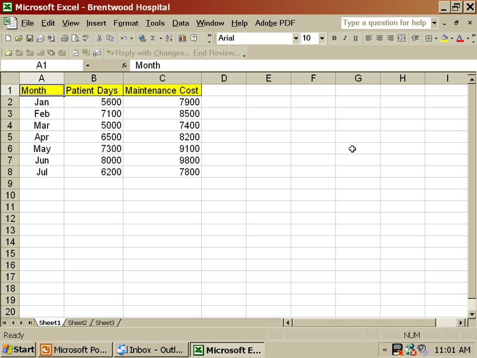
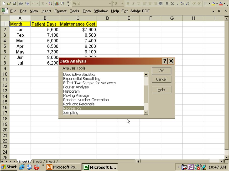
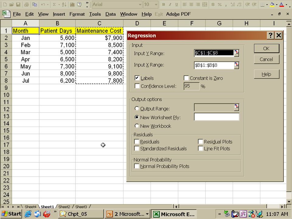
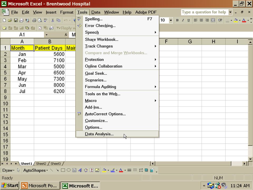
April 15, 2017
Brentline Hospital Patient Data
Month
Activity Level: Patient Days
Maintenance Cost Incurred
January
5,600
$7,900
February
7,100
8,500
March
5,000
7,400
April
6,500
8,200
May
7,300
9,100
June
8,000
9,800
July
6,200
7,800
Textbook Example
Dr. Fred Barbee

31. Cost Behavior: Analysis and Use
April 15, 2017
Dr. Fred Barbee

32. Cost Behavior: Analysis and Use
April 15, 2017
Dr. Fred Barbee

33. Cost Behavior: Analysis and Use
April 15, 2017
Dr. Fred Barbee

34. Cost Behavior: Analysis and Use
April 15, 2017
Dr. Fred Barbee

35. From Algebra . . .
If we know any two points on a line, we can determine the slope of that line.

36. High-Low Method
A non-statistical method whereby we examine two points out of a set of data . . .
The high point; and
The low point

37. High-Low Method
Using these two points, we determine the equation for that line . . .
The intercept; and
The Slope parameters
y = a + bX

38. High-Low Method To get the variable costs . . .
We compare the difference in costs between the two periods to
The difference in activity between the two periods.

39. Cost Behavior: Analysis and Use
April 15, 2017
Brentline Hospital Patient Data
Month
Activity Level: Patient Days
Maintenance Cost Incurred
January
5,600
$7,900
February
7,100
8,500
March
5,000
7,400
April
6,500
8,200
May
7,300
9,100
June
8,000
9,800
July
6,200
7,800
Low
High
Textbook Example
Dr. Fred Barbee

40. High June 8,000 $9,800 Low March 5,000 7,400 Difference 3,000 $2,400
High/ Low
Month
Patient Days
Maint. Cost
High
June
8,000
$9,800
Low
March
5,000
7,400
Difference
3,000
$2,400

41. (Y2 - Y1) V = ------------ (X2 - X1) Change in Cost
Change in Activity
(Y2 - Y1)
V =
(X2 - X1)

42. Divided by the change in activity
Calculate the Variable Rate
High/ Low
Month
Patient Days
Maint. Cost
The Change in Cost
High
June
8,000
$9,800
Low
March
5,000
7,400
Divided by the change in activity
Difference
3,000
$2,400

43. $2,400 V = ------------ 3,000 = $0.80 Per Unit Change in Cost
Change in Activity
$2,400
V =
3,000
= $0.80 Per Unit

44. Total Cost (TC) = FC + VC - FC = - TC + VC FC = TC - VC
Calculate Fixed Costs
Total Cost (TC) = FC + VC
- FC = - TC + VC
FC = TC - VC

45. FC = $9,800 - (8,000 x $0.80) = $3,400 Calculate Fixed Costs
Using June
FC = TC - VC
FC = $9,800 - (8,000 x $0.80)
= $3,400

46. FC = $7,400 - (5,000 x $0.80) = $3,400 Calculate Fixed Costs
Using March
FC = TC - VC
FC = $7,400 - (5,000 x $0.80)
= $3,400

47. The Cost Formula
y = a + bx
TC = $3,400 + $0.80X

48. Cost Behavior: Analysis and Use
April 15, 2017
Month
Activity Level: Patient Days
Maintenance Cost Incurred
January
5,600
$7,900
February
7,100
8,500
March
5,000
7,400
April
6,500
8,200
May
7,300
9,100
June
8,000
9,800
July
6,200
7,800
We have taken “Total Costs” which is a mixed cost and we have separated it into its VC and FC components.
Dr. Fred Barbee

49. So what. You say. Thank you for asking
So what? You say! Thank you for asking! Now I can use this formula for planning purposes. For example, what if I believe my activity level will be 6,325 patient days in February. What would I expect my total maintenance cost to be?

50. What is the estimated total cost if the activity level for February is expected to be 6,325 patient days?
Y = a + bx
TC = $3, ,325 x $0.80
TC = $8,460

51. Some Important Considerations
We have used historical cost to arrive at the cost equation.
Therefore, we have to be careful in how we use the formula.
Never forget the relevant range.

52. Cost Behavior: Analysis and Use
April 15, 2017
5,000
8,000
Relevant Range $
5,000 to 8,000 activity level
Volume (Activity Base)
Dr. Fred Barbee

53. Strengths of High-Low Method
Simple to use
Easy to understand

54. Weaknesses of High-Low
Only two data points are used in the analysis.
Can be problematic if either (or both) high or low are extreme (i.e., Outliers).

55. Extreme values - not necessarily representative. . . . . . . . . . . . . . .
Representative High/Low Values

56. Weaknesses of High-Low
Other months may not yield the same formula.

57. FC = $8,500 - (7,100 x $0.80) = $2,820 Calculate Fixed Costs
Using February
FC = TC - VC
FC = $8,500 - (7,100 x $0.80)
= $2,820

58. FC = $7,800 - (6,200 x $0.80) = $2,840 Calculate Fixed Costs
Using July
FC = TC - VC
FC = $7,800 - (6,200 x $0.80)
= $2,840

59. Regression Analysis
A statistical technique used to separate mixed costs into fixed and variable components.
All observations are used to fit a regression line which represents the average of all data points.

60. Cost Behavior: Analysis and Use
April 15, 2017
Regression Analysis
Requires the simultaneous solution of two linear equations
So that the squared deviations from the regression line of each of the plotted points cancel out (are equal to zero).
Dr. Fred Barbee

61. Cost Actual Y Estimated y
Error
Estimated y
The objective is to find values of a and b in the equation y = a + bX that minimize
Production

62. The equation for a linear function (straight line) with one independent variable is . . .
y = a + bX
Where:
y = The Dependent Variable a = The Constant term (Intercept) b = The Slope of the line X = The Independent variable

63. The Dependent Variable The Independent Variable
The equation for a linear function (straight line) with one independent variable is . . .
The Dependent Variable
y = a + bX
Where:
y = The Dependent Variable a = The Constant term (Intercept) b = The Slope of the line X = The Independent variable
The Independent Variable

64. Cost Behavior: Analysis and Use
April 15, 2017
Regression Analysis
With this equation and given a set of data.
Two simultaneous linear equations can be developed that will fit a regression line to the data.
Dr. Fred Barbee

65. Least-Squares Equations
Where: a = Fixed cost b = Variable cost n = Number of observations X = Activity measure (Hours, etc.) Y = Total cost

66. Estimating the Regression Line

72. Fixed Costs
Variable Costs

73. This is referred to as a “goodness of fit” measure.
R2, the Coefficient of Determination is the percentage of variability in the dependent variable being explained by the independent variable.
This is referred to as a “goodness of fit” measure.

74. R, the Coefficient of Correlation is square root of R2
R, the Coefficient of Correlation is square root of R2. Can range from -1 to +1. Positive correlation means the variables move together. Negative correlation means they move in opposite directions.

75. Cost Behavior: Analysis and Use
April 15, 2017
Comparison of Methods
Method
Fixed Cost
Variable Cost
High-Low
$3,400
$0.80
Scattergraph
$3,300
$0.79
Regression
$3,431
$0.76
Dr. Fred Barbee

76. Coefficient of Determination
Cost Behavior: Analysis and Use
April 15, 2017
Coefficient of Determination
R2 is the percentage of variability in the dependent variable that is explained by the independent variable.
Dr. Fred Barbee

77. Coefficient of Determination
Cost Behavior: Analysis and Use
April 15, 2017
Coefficient of Determination
This is a measure of goodness-of-fit.
The higher the R2, the better the fit.
Dr. Fred Barbee

78. Coefficient of Determination
Cost Behavior: Analysis and Use
April 15, 2017
Coefficient of Determination
The higher the R2, the more variation (in the dependent variable) being explained by the independent variable.
Dr. Fred Barbee

79. Coefficient of Determination
Cost Behavior: Analysis and Use
April 15, 2017
Coefficient of Determination
R2 ranges from 0 to 1.0
Good Vs. Bad R2s is relative.
There is no magic cutoff
Dr. Fred Barbee

80. Coefficient of Correlation
Cost Behavior: Analysis and Use
April 15, 2017
Coefficient of Correlation
The relationship between two variables can be described by a correlation coefficient.
The coefficient of correlation is the square root of the coefficient of determination.
Dr. Fred Barbee

81. Coefficient of Correlation
Cost Behavior: Analysis and Use
April 15, 2017
Coefficient of Correlation
Provides a measure of strength of association between two variables.
The correlation provides an index of how closely two variables “go together.”
Dr. Fred Barbee

82. Cost Behavior: Analysis and Use
April 15, 2017
Positive Correlation
Machine Hours
Utility Costs
Machine Hours
Utility Costs
r approaches +1
Dr. Fred Barbee

83. Cost Behavior: Analysis and Use
April 15, 2017
r approaches +1
Dr. Fred Barbee

84. Cost Behavior: Analysis and Use
April 15, 2017
r Equals +1
Dr. Fred Barbee

85. Cost Behavior: Analysis and Use
April 15, 2017
Negative Correlation
Hours of Safety Training
Industrial Accidents
Hours of Safety Training
Industrial Accidents
r approaches -1
Dr. Fred Barbee

86. Cost Behavior: Analysis and Use
April 15, 2017
r approaches -1
Dr. Fred Barbee

87. Cost Behavior: Analysis and Use
April 15, 2017
r Equals -1
Dr. Fred Barbee

88. Cost Behavior: Analysis and Use
April 15, 2017
No Correlation
Hair Length
202 Grade
Hair Length
202 Grade
r ~ 0
Dr. Fred Barbee

89. Cost Behavior: Analysis and Use
April 15, 2017
Dr. Fred Barbee

90. Cost Behavior: Analysis and Use
April 15, 2017
Dr. Fred Barbee

92. Cost Behavior: Analysis and Use
April 15, 2017
Dr. Fred Barbee

93. Cost Behavior: Analysis and Use
April 15, 2017
Dr. Fred Barbee

94. Cost Behavior: Analysis and Use
April 15, 2017
Dr. Fred Barbee