1. Geometric aspects of variability

2. A simple building system could be schematically conceived as a spatial allocation of cells, each cell characterized by an attribute which accepts different values. Different states of the system, each state determined by a different attribute value assignment to the system's cells, represent different building constructions attainable by the system.

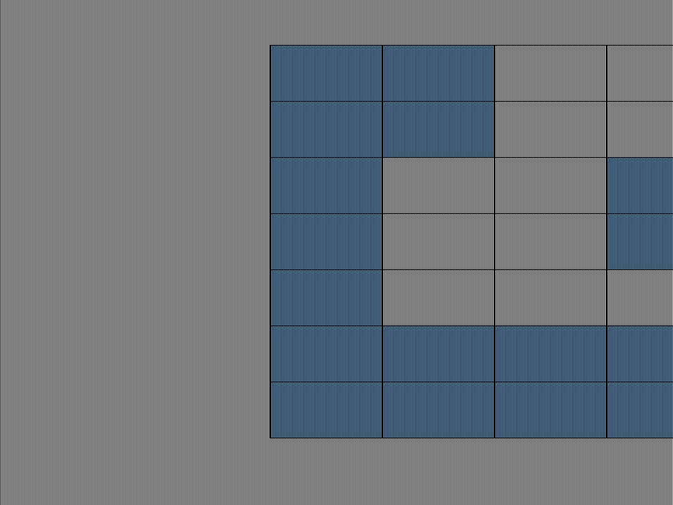
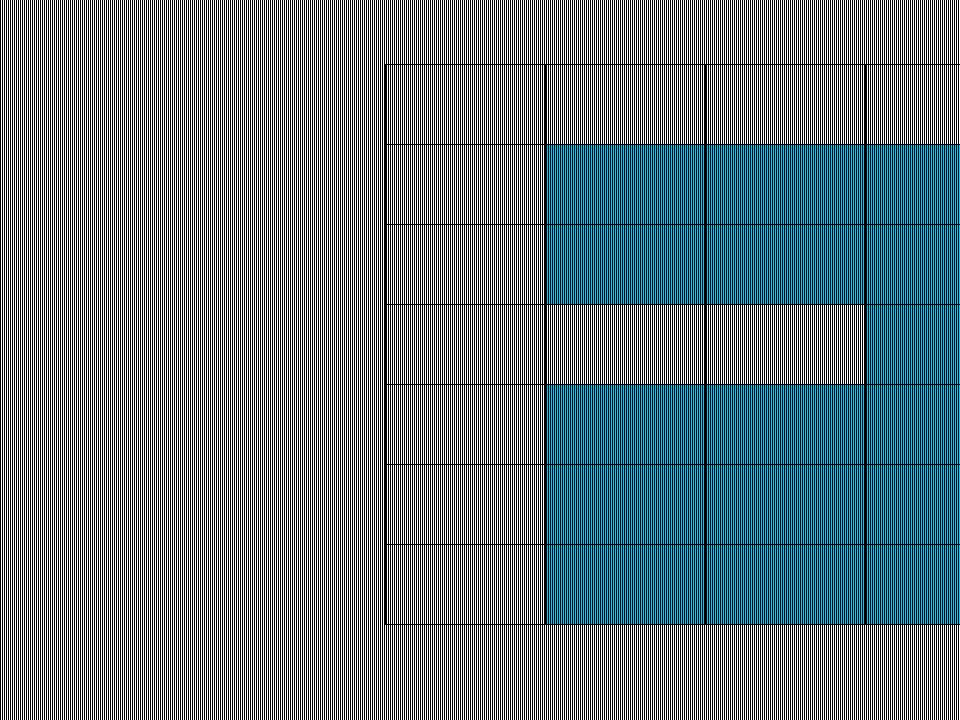
3. For instance consider a square grid, each cell of which is characterized by the binary attribute "built space", where the value 1 denotes "built" while the value 0 denotes "not built". Then, different states of the system (visualized here by representing 0 with white color and 1 with blue color) could represent different architectural plans.

6. In this case the system has 2 N possible states, where N is the number of the cells. More generally, a system of N cells—where the characteristic cell's attribute accepts W different possible values—has W N possible states. The number of the possible states will be referred to as the "variability" of the system. Considering variability as a desired system's property independent from every particular application case, we would like to find a configuration of cells on the Plane—the latter viewed as the terrain of an architectural plan—which maximizes variability density, i.e. variability per area unit. Given W (the number of possible states of a cell), variability density increases with the number of cells per area unit. Then, an obvious way to maximize variability is to minimize the cell's size. However this size could be determined by either ergonomic, or architectural, or urban factors. These factors fall into a general model which can be extracted by the following observation: Of course, due to architectural constraints, only a fraction of the possible system’s states constitute valid architectural plans. However, the expected number of these states is heavily depended on variability.

7. R C R D Suppose that each cell accommodates an elementary space-use facility, the latter represented as a pair (C, R), where C is the geometric center of the facility and R is the radius specifying the facility's range. Depending on the scale of the facility, R could range from a few feet (furniture scale) to a few hundreds of feet (urban scale). What is important is that, given the scale, a minimum R is determined, while the minimum center-to-center distance is defined as D = 2  R.

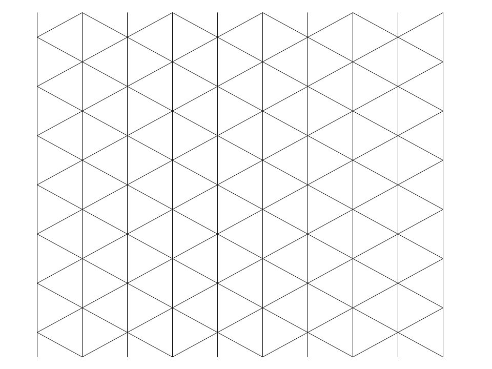
8. D It is known that if points having a minimum allowed distance between each other are to be allocated on the Plane, then the allocation having the maximum number of points per area unit is achieved if points constitute vertices of an equilateral triangular lattice where the side of a triangle equals the minimum allowed distance.

9. The boundaries between cells are given by the dual grid i.e. the grid of which the edges are perpendicular bisectors of the edges of the lattice. As a consequence, the cells occur as equal regular hexagons. An hexagonal grid has approximately 15% more cells per area unit than a square grid having the same center-to-center cell distance. This increases variability density by an exponential factor of 1.15.

10. Considering different assignments of a binary value on grid cells as different architectural plans is of course a rough approximation.

11. Then, by definition the variability density is W N, where W is the number of the possible states of a boundary (this includes the number of object types plus the "no object" case) and N is the number of boundaries per area unit. Even according to the new approach to variability, the hexagonal grid maximizes variability density: it includes approximately 73% more cell boundaries per area unit than a square grid having the same center-to-center cell distance. This increases variability density by an exponential factor of 1.73. In fact the structural elements of our system could be objects (thick or thin panels, doors, windows etc.) which can be placed at the cell-to-cell boundaries.

12. 3D LatticeCell of the dual grid If the system is extended in three dimensions, then the facilities' centers form a 3D lattice where neighboring centers are connected. Dualism occurs if each connection is replaced by its perpendicular bisector plane. Then the planar segments that surround each center form a polyhedron which constitutes cell of a 3D grid. The densest 3D grid, i.e. the 3D grid having the largest number of cells per volume unit given a minimum allowed center-to-center distance, is the grid of which the cells are equal rhombic dodecahedrons. This grid also exhibits the maximum variability density in three dimensions.

13. 3D LatticeCell of the dual grid Another dense 3D grid, potentially offering better architectural properties, is the grid of which the cells are equal truncated octahedrons. These grids, as well as the 2D hexagonal grid, have two properties important for their potential architectural applications: they are left fixed by translation and rotation. This retains homogeneity and isotropy in the large scale. Consequently, the possibilities of architectural manipulation of the space are the same for a uniformly distributed set of positions and directions. However 3D architectural space is not isotropic, as it is orientated by the gravity vector. Due to this anisotropy, human activities are more intensive on horizontal levels than on the vertical direction. As a consequence, a 3D grid should be anisotropic, exhibiting maximum variability density according to horizontal levels.

14. 3D LatticeCell of the dual grid An obvious—although not necessarily best—solution derives from a 3D lattice where the facilities' centers form equilateral triangular 2D lattices on successive horizontal planes (this makes sure maximum variability density on these planes), while homologous centers lying on successive planes are connected vertically. Then the dual grid's cell is an hexagonal prism.

15. Any horizontal section of this grid reveals the familiar 2D hexagonal grid. However a building system based on the hexagonal grid does not scale well. Consider for instance the larger-scale spatial module appearing in red color. This module could correspond to an architectural-scale unit, if hexagonal cells correspond to furniture-scale units. The particular module cannot be constructed by the system, as the latter does not provide the necessary elementary boundaries. A system-consistent construction can only approximate this module by an unnecessary waste in both boundary length and complexity.

17. If we connect each vertex of each hexagon with the hexagon's center we get an equilateral triangular fine-grained construction grid where structural elements can be placed. The hexagonal grid is included in the new grid, which means that every construction available by the former grid is also available by the latter one.

18. However, under the proper architectural constraints which make sure non violation of the minimum allowed distance between facilities' centers, the new grid could support additional constructions …

19. … including the spatial module presented before. As a consequence the new grid allows scaling of the construction units, while significantly increases variability density.

20. Now let us see a vertical section of the 3D lattice formed by the facilities' centers. Here, horizontal lines represent horizontal Planes, each Plane having an equilateral triangular grid, while vertical lines represent columns of vertical connections. Dual polyhedrons appear in this section as rectangles.

22. Suppose that it is allowed to alter the 3D lattice by both shifting vertically any subset of columns by half the height of a vertical connection and creating new connections as required to retain vertical symmetry. Then a 3D lattice with K columns has 2 K possible states. Substitution of a horizontal connection by two oblique connections results in breaking the respective vertical surface of a dual polyhedron in two oblique surfaces.

23. A possible state of the 3D Lattice Respective state of dual grid’s cells As a consequence, a dual polyhedron could range from a prism, where all but the horizontal surfaces are vertical (if all neighbor columns have the same shift state as the polyhedron's column), …

24. A possible state of the 3D Lattice Respective states of dual grid’s cells … to a diamond-shaped polyhedron, where all vertical surfaces have been substituted by pairs of oblique surfaces (if all neighbor columns have different shift state than the polyhedron's column). The possibility to shift columns of the 3D lattice does not hurt homogeneity at the system level, as it is uniformly distributed in space. Variability is multiplied by the number of the possible shift states of the 3D lattice. Specifically, given a region available for building construction, variability is multiplied by 2 K where K is the number of lattice's columns that intersect the region. The succession of the dual grids of the possible states of the 3D lattice forms a fixed fine-grained 3D grid, of which the elementary planar segments result from the intersection of the planar segments of the successive grids. The fine-grained grid could be considered as the construction grid of elementary planar segments which should be placed according to system-level constraints.

25. Continued in Section_3_EN.PPS