Download presentation
Presentation is loading. Please wait.

1
1 Dynamic Programming Jose Rolim University of Geneva

2
Dynamic ProgrammingJose Rolim2 Fibonacci sequence Fibonacci sequence: 0, 1, 1, 2, 3, 5, 8, 13, 21, … F i = i if i 1 F i = F i-1 + F i-2 if i 2 Solved by a recursive program:

3
Dynamic ProgrammingJose Rolim3 Fibonacci sequence Complexity: O(4**n) Much replicated computation is done. It should be solved by a simple loop. ORDERING IS ESSENTIAL !!!!!!!!

4
Dynamic ProgrammingJose Rolim4 Binomial coefficients (x + y) 2 = x 2 + 2xy + y 2, coefficients are 1,2,1 (x + y) 3 = x 3 + 3x 2 y + 3xy 2 + y 3, coefficients are 1,3,3,1 (x + y) 4 = x 4 + 4x 3 y + 6x 2 y 2 + 4xy 3 + y 4, coefficients are 1,4,6,4,1 (x + y) 5 = x 5 + 5x 4 y + 10x 3 y 2 + 10x 2 y 3 + 5xy 4 + y 5, coefficients are 1,5,10,10,5,1
 2 = x 2 + 2xy + y 2, coefficients are 1,2,1 (x + y) 3 = x 3 + 3x 2 y + 3xy 2 + y 3, coefficients are 1,3,3,1 (x + y) 4 = x 4 + 4x 3 y + 6x 2 y 2 + 4xy 3 + y 4, coefficients are 1,4,6,4,1 (x + y) 5 = x 5 + 5x 4 y + 10x 3 y x 2 y 3 + 5xy 4 + y 5, coefficients are 1,5,10,10,5,1")
5
Dynamic ProgrammingJose Rolim5 Binomial coefficients The n+1 coefficients can be computed for (x + y) n according to the formula c(n, i) = n! / (i! * (n – i)!) for each of i = 0..n The repeated computation of all the factorials gets to be expensive We can use smart ordering to save the factorials as we go
!) for each of i = 0..n The repeated computation of all the factorials gets to be expensive We can use smart ordering to save the factorials as we go.")
6
Dynamic ProgrammingJose Rolim6 Solution: n c(n,0) c(n,1) c(n,2) c(n,3) c(n,4) c(n,5) c(n,6) 0 1 1 1 1 2 1 2 1 3 1 3 3 1 4 1 4 6 4 1 5 1 5 10 10 5 1 6 1 6 15 20 15 6 1 Each row depends only on the preceding row Only linear space and quadratic time are needed This algorithm is known as Pascal’s Triangle
 c(n,1) c(n,2) c(n,3) c(n,4) c(n,5) c(n,6) 0 1 Each row depends only on the preceding row Only linear space and quadratic time are needed This algorithm is known as Pascal’s Triangle")
7
Dynamic ProgrammingJose Rolim7 Algorithm in Java public static int binom(int n, int m) { int[ ] b = new int[n + 1]; b[0] = 1; for (int i = 1; i 0; j--) { b[j] += b[j – 1]; } } return b[m]; }
![Dynamic ProgrammingJose Rolim7 Algorithm in Java public static int binom(int n, int m) { int[ ] b = new int[n + 1]; b[0] = 1; for (int i = 1; i 0; j--) { b[j] += b[j – 1]; } } return b[m]; }](http://images.slideplayer.com/15/4527801/slides/slide_7.jpg "Dynamic ProgrammingJose Rolim7 Algorithm in Java public static int binom(int n, int m) { int[ ] b = new int[n + 1]; b[0] = 1; for (int i = 1; i 0; j--) { b[j] += b[j – 1]; } } return b[m]; }")
8
Dynamic ProgrammingJose Rolim8 Making change Set of coins: 25, 10, 5 and 1 To find the minimum number of coins to make any amount, the greedy method always works At each step, just choose the largest coin that does not overshoot the desired amount: 31¢=25

9
Dynamic ProgrammingJose Rolim9 Making change The greedy method would not work if we did not have 5¢ coins For 31 cents, the greedy method gives seven coins (25+1+1+1+1+1+1), but we can do it with four (10+10+10+1) The greedy method also would not work if we had a 21¢ coin For 63 cents, the greedy method gives six coins (25+25+10+1+1+1), but we can do it with three (21+21+21)
, but we can do it with four ( ) The greedy method also would not work if we had a 21¢ coin For 63 cents, the greedy method gives six coins ( ), but we can do it with three ( )")
10
Dynamic ProgrammingJose Rolim10 More general problem How can we find the minimum number of coins for any given coin set? For the following examples, we will assume coins in the following denominations: 1¢ 5¢ 10¢ 21¢ 25¢ We’ll use 63¢ as our goal

11
Dynamic ProgrammingJose Rolim11 Simple solution We always need a 1¢ coin, otherwise no solution exists for making one cent To make K cents: If there is a K-cent coin, then that one coin is the minimum Otherwise, for each value i < K, Find the minimum number of coins needed to make i cents Find the minimum number of coins needed to make K - i cents Choose the i that minimizes this sum

12
Dynamic ProgrammingJose Rolim12 Divide and conquer solution This algorithm can be viewed as divide- and-conquer, or as brute force This solution is very recursive It requires exponential work It is infeasible to solve for 63¢

13
Dynamic ProgrammingJose Rolim13 Another solution We can reduce the problem recursively by choosing the first coin, and solving for the amount that is left For 63¢: One 1¢ coin plus the best solution for 62¢ One 5¢ coin plus the best solution for 58¢ One 10¢ coin plus the best solution for 53¢ One 21¢ coin plus the best solution for 42¢ One 25¢ coin plus the best solution for 38¢ Choose the best solution from among the 5 given above Instead of solving 62 recursive problems, we solve 5 This is still a very expensive algorithm

14
Dynamic ProgrammingJose Rolim14 A dynamic programming solution Idea: Solve first for one cent, then two cents, then three cents, etc., up to the desired amount Save each answer in an array !

15
Dynamic ProgrammingJose Rolim15 For instance For each new amount N, compute all the possible pairs of previous answers which sum to N For example, to find the solution for 13¢, First, solve for all of 1¢, 2¢, 3¢,..., 12¢ Next, choose the best solution among: Solution for 1¢ + solution for 12¢ Solution for 2¢ + solution for 11¢ Solution for 3¢ + solution for 10¢ Solution for 4¢ + solution for 9¢ Solution for 5¢ + solution for 8¢ Solution for 6¢ + solution for 7¢

16
Dynamic ProgrammingJose Rolim16 Example Suppose coins are 1¢, 3¢, and 4¢ There’s only one way to make 1¢ (one coin) To make 2¢, try 1¢+1¢ (one coin + one coin = 2 coins) To make 3¢, just use the 3¢ coin (one coin) To make 4¢, just use the 4¢ coin (one coin) To make 5¢, try 1¢ + 4¢ (1 coin + 1 coin = 2 coins) 2¢ + 3¢ (2 coins + 1 coin = 3 coins) The first solution is better, so best solution is 2 coins To make 6¢, try 1¢ + 5¢ (1 coin + 2 coins = 3 coins) 2¢ + 4¢ (2 coins + 1 coin = 3 coins) 3¢ + 3¢ (1 coin + 1 coin = 2 coins) – best solution Etc.
 To make 2¢, try 1¢+1¢ (one coin + one coin = 2 coins) To make 3¢, just use the 3¢ coin (one coin) To make 4¢, just use the 4¢ coin (one coin) To make 5¢, try 1¢ + 4¢ (1 coin + 1 coin = 2 coins) 2¢ + 3¢ (2 coins + 1 coin = 3 coins) The first solution is better, so best solution is 2 coins To make 6¢, try 1¢ + 5¢ (1 coin + 2 coins = 3 coins) 2¢ + 4¢ (2 coins + 1 coin = 3 coins) 3¢ + 3¢ (1 coin + 1 coin = 2 coins) – best solution Etc.")
17
Dynamic ProgrammingJose Rolim17 Comparison The first algorithm is recursive, with a branching factor of up to 62 Possibly the average branching factor is somewhere around half of that (31) The algorithm takes exponential time, with a large base The second algorithm is much better—it has a branching factor of 5 This is exponential time, with base 5 The dynamic programming algorithm is O(N*K), where N is the desired amount and K is the number of different kinds of coins
 The algorithm takes exponential time, with a large base The second algorithm is much better—it has a branching factor of 5 This is exponential time, with base 5 The dynamic programming algorithm is O(N*K), where N is the desired amount and K is the number of different kinds of coins")
18
Dynamic ProgrammingJose Rolim18 Comparison with divide and conquer Divide-and-conquer algorithms split a problem into separate subproblems, solve the subproblems, and combine the results for a solution to the original problem Example: Quicksort Example: Mergesort Example: Binary search Divide-and-conquer algorithms can be thought of as top- down algorithms In contrast, a dynamic programming algorithm proceeds by solving small problems, then combining them to find the solution to larger problems

19
Dynamic ProgrammingJose Rolim19 More formally Let: Coin i has value di, we have to give N back Consider c[i,j] as the minimum number of coins to pay j with coins from 1 to i. Solution is c[n,N] c[i,0]=0 c[i,j]=min[c[i-1,j],1+c[i,j-di]] Ordering ???
![Dynamic ProgrammingJose Rolim19 More formally Let: Coin i has value di, we have to give N back Consider c[i,j] as the minimum number of coins to pay j with coins from 1 to i.](http://images.slideplayer.com/15/4527801/slides/slide_19.jpg " Solution is c[n,N] c[i,0]=0 c[i,j]=min[c[i-1,j],1+c[i,j-di]] Ordering .")
20
Dynamic ProgrammingJose Rolim20 Example: N=8 and 1,4,6 coins N= 0 1 2 3 4 5 6 7 8 di=1 0 1 2 3 4 5 6 7 8 di=4 0 1 2 3 1 2 3 4 2 di=6 0 1 2 3 1 2 1 2 2 For instance c[3,8]= min of c[2,8]= 2 and 1+c[3,2-d3]=3. Thus, 2.
![Dynamic ProgrammingJose Rolim20 Example: N=8 and 1,4,6 coins N= di= di= di= For instance c[3,8]= min of c[2,8]= 2 and 1+c[3,2-d3]=3.](http://images.slideplayer.com/15/4527801/slides/slide_20.jpg "Thus, 2..")
21
Dynamic ProgrammingJose Rolim21 Formal version Function coins(N) Array d[1...n] Array c[1..n,0..N] For i=1 to n do c[1,0]=0 For i=1 to n do For j=1 to N do c[i,j]=if i=1 and j <di then inf else if i=1 then 1+c[1,j-d1] else if j<di then c[i-1,j] else min{c[i-1,j], 1+c[i,j-di]} Return c[n,N]
![Dynamic ProgrammingJose Rolim21 Formal version Function coins(N) Array d[1...n] Array c[1..n,0..N] For i=1 to n do c[1,0]=0 For i=1 to n do For j=1 to N do c[i,j]=if i=1 and j <di then inf else if i=1 then 1+c[1,j-d1] else if j<di then c[i-1,j] else min{c[i-1,j], 1+c[i,j-di]} Return c[n,N]](http://images.slideplayer.com/15/4527801/slides/slide_21.jpg "Dynamic ProgrammingJose Rolim21 Formal version Function coins(N) Array d[1...n] Array c[1..n,0..N] For i=1 to n do c[1,0]=0 For i=1 to n do For j=1 to N do c[i,j]=if i=1 and j <di then inf else if i=1 then 1+c[1,j-d1] else if j<di then c[i-1,j] else min{c[i-1,j], 1+c[i,j-di]} Return c[n,N]")
22
Dynamic ProgrammingJose Rolim22 Principle of optimality Dynamic programming is a technique for finding an optimal solution The principle of optimality applies if the optimal solution to a problem always contains optimal solutions to all subproblems Example: Consider the problem of making N¢ with the fewest number of coins Either there is an N¢ coin, or The set of coins making up an optimal solution for N¢ can be divided into two nonempty subsets, n 1 ¢ and n 2 ¢ If either subset, n 1 ¢ or n 2 ¢, can be made with fewer coins, then clearly N¢ can be made with fewer coins, hence solution was not optimal

23
Dynamic ProgrammingJose Rolim23 Principle of optimality The principle of optimality holds if Every optimal solution to a problem contains... ...optimal solutions to all subproblems The principle of optimality does not say If you have optimal solutions to all subproblems... ...then you can combine them to get an optimal solution Example: In US coinage, The optimal solution to 7¢ is 5¢ + 1¢ + 1¢, and The optimal solution to 6¢ is 5¢ + 1¢, but The optimal solution to 13¢ is not 5¢ + 1¢ + 1¢ + 5¢ + 1¢ But there is some way of dividing up 13¢ into subsets with optimal solutions (say, 11¢ + 2¢) that will give an optimal solution for 13¢ Hence, the principle of optimality holds for this problem
 that will give an optimal solution for 13¢ Hence, the principle of optimality holds for this problem.")
24
Dynamic ProgrammingJose Rolim24 Dynamic programming Ordering + Principle of optimality

25
Dynamic ProgrammingJose Rolim25 Matrix multiplication Given matrix A (size: p q) and B (size: q r) Compute C = A B A and B must be compatible Time to compute C (number of scalar multiplications) = pqr
 and B (size: q r) Compute C = A B A and B must be compatible Time to compute C (number of scalar multiplications) = pqr")
26
Dynamic ProgrammingJose Rolim26 Matrix-chain Multiplication Different ways to compute C Matrix multiplication is associative So output will be the same However, time cost can be very different

27
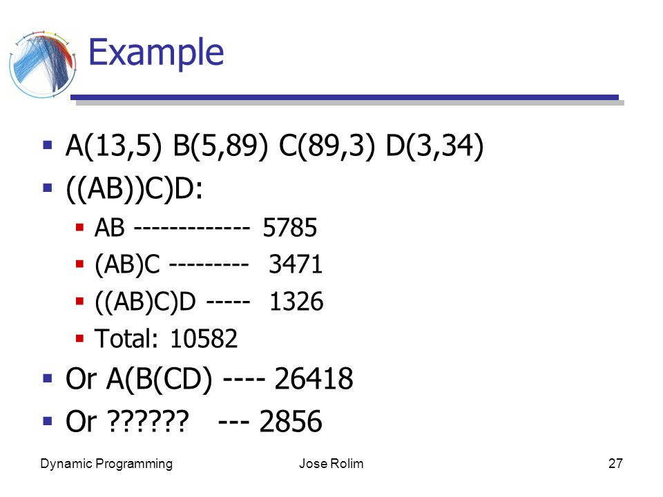
Dynamic ProgrammingJose Rolim27 Example A(13,5) B(5,89) C(89,3) D(3,34) ((AB))C)D: AB ------------- 5785 (AB)C --------- 3471 ((AB)C)D ----- 1326 Total: 10582 Or A(B(CD) ---- 26418 Or ?????? --- 2856
28
Dynamic ProgrammingJose Rolim28 Problem Definition fully parenthesize the product in a way that minizes the number of scalar multiplications ( ( ) ( ) ) ( ( ) ( ( ) ( ( ) ( ) ) ) ) Number of parenthesizations: exponential
 ( ) ) ( ( ) ( ( ) ( ( ) ( ) ) ) ) Number of parenthesizations: exponential")
29
Dynamic ProgrammingJose Rolim29 Extract the Problem Define the problem: MM(i, j) let m(i,j) = smallest number of scalar multiplications Goal: MM(1, n) (with m(1,n) )
 let m(i,j) = smallest number of scalar multiplications Goal: MM(1, n) (with m(1,n) )")
30
Dynamic ProgrammingJose Rolim30 Structure of Optimal Parenthesization Given MM(i, j): ( ( ) ( ) ) ( ( ) ( ( ) ( ( ) ( ) ) ) ) Imagine we take the leftmost left-parenthesis and its pairing right-parenthesis Break MM(i,j) into two parts Suppose break at k’th position Subproblems: MM(i,k), MM(k+1, j) Optimal substructure property Where to break
: ( ( ) ( ) ) ( ( ) ( ( ) ( ( ) ( ) ) ) ) Imagine we take the leftmost left-parenthesis and its pairing right-parenthesis Break MM(i,j) into two parts Suppose break at k’th position Subproblems: MM(i,k), MM(k+1, j) Optimal substructure property Where to break")
31
Dynamic ProgrammingJose Rolim31 A Recursive Solution Base case for m[i,j] i = j, m[ i, i ] = 0 Otherwise, if it’s broken at i ≤ k < j
![Dynamic ProgrammingJose Rolim31 A Recursive Solution Base case for m[i,j] i = j, m[ i, i ] = 0 Otherwise, if it’s broken at i ≤ k < j](http://images.slideplayer.com/15/4527801/slides/slide_31.jpg "Dynamic ProgrammingJose Rolim31 A Recursive Solution Base case for m[i,j] i = j, m[ i, i ] = 0 Otherwise, if it’s broken at i ≤ k < j")
32
Dynamic ProgrammingJose Rolim32 Compute Optimal Cost How to do bottom-up?

33
Dynamic ProgrammingJose Rolim33 Construct Opt-solution Remember the breaking position chosen for each table entry. Total time complexity: Each table entry: Number of choices: O(j-i) Each choice: O(1) O(n^3) running time
 Each choice: O(1) O(n^3) running time.")
34
Dynamic ProgrammingJose Rolim34 Remarks More than constant choices The order to build table

Similar presentations


 The General Technique (§5.3.2) 0-1 Knapsack Problem (§5.3.3)>")


 The General Technique (§5.3.2) 0-1 Knapsack Problem (§5.3.3)>")
![1 Dynamic Programming Andreas Klappenecker [based on slides by Prof. Welch]](/16/5142786/big_thumb.jpg "1 Dynamic Programming Andreas Klappenecker [based on slides by Prof. Welch]>")