1. Computer Vision – Image Representation (Histograms)
(Slides borrowed from various presentations)

2. Image representations
Templates
Intensity, gradients, etc.
Histograms
Color, texture, SIFT descriptors, etc.

3. Image Representations: Histograms
Global histogram
Represent distribution of features
Color, texture, depth, …
Space Shuttle Cargo Bay
Images from Dave Kauchak

4. Image Representations: Histograms
Histogram: Probability or count of data in each bin
Joint histogram
Requires lots of data
Loss of resolution to avoid empty bins
Marginal histogram
Requires independent features
More data/bin than joint histogram
Images from Dave Kauchak

5. Image Representations: Histograms
Clustering
EASE Truss Assembly
Use the same cluster centers for all images
Space Shuttle Cargo Bay
Images from Dave Kauchak

6. Computing histogram distance
Histogram intersection (assuming normalized histograms)
Chi-squared Histogram matching distance
Cars found by color histogram matching using chi-squared

7. Histograms: Implementation issues
Quantization
Grids: fast but applicable only with few dimensions
Clustering: slower but can quantize data in higher dimensions
Matching
Histogram intersection or Euclidean may be faster
Chi-squared often works better
Earth mover’s distance is good for when nearby bins represent similar values
Few Bins
Need less data
Coarser representation
Many Bins
Need more data
Finer representation

8. What kind of things do we compute histograms of?
Color
Texture (filter banks or HOG over regions)
L*a*b* color space
HSV color space

9. What kind of things do we compute histograms of?
Histograms of oriented gradients
SIFT – Lowe IJCV 2004

10. Orientation Normalization
Compute orientation histogram
Select dominant orientation
Normalize: rotate to fixed orientation
[Lowe, SIFT, 1999] 2 p
T. Tuytelaars, B. Leibe

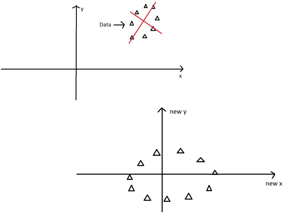
11. But what about layout?
All of these images have the same color histogram

12. Spatial pyramid
Compute histogram in each spatial bin

13. Spatial pyramid representation
Extension of a bag of features
Locally orderless representation at several levels of resolution
level 0
Lazebnik, Schmid & Ponce (CVPR 2006)

14. Spatial pyramid representation
Extension of a bag of features
Locally orderless representation at several levels of resolution
level 1
level 0
Lazebnik, Schmid & Ponce (CVPR 2006)

15. Spatial pyramid representation
Extension of a bag of features
Locally orderless representation at several levels of resolution
level 2
level 0
level 1
Lazebnik, Schmid & Ponce (CVPR 2006)

16. Feature Vectors & Representation Power
How to analyze the information content in my features?
Is there a way to visualize the representation power of my features?

17. Mean, Variance, Covariance and Correlation

18. Covariance Explained

19. Covariance Cheat Sheet

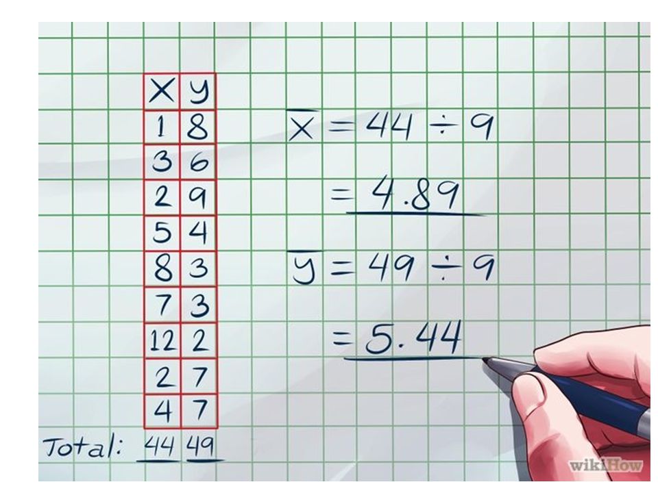
20. Organize your data into a set of (x, y)
First we need to calculate the means of both x and y independently.

22. Plug your variables into the formula
Now, you have everything you need to find the covariance of x and y. Plug your value for n, your x and y averages, and your individual x and y values into the appropriate spaces to get the covariance of x and y -> Cov(x, y)

23. Covariance is unbounded
Depending on the different units of x and y, the range of values that x and y take can be far away from each other.
In order to normalize the covariance value, we can use the below formula:
This is called Correlation.

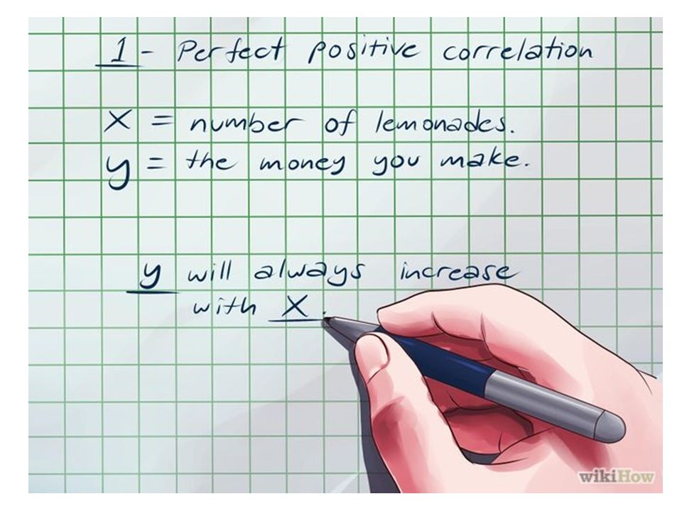
24. Know that a correlation of 1 indicates perfect positive correlation.
When it comes to correlations, your answers will always be between 1 and -1. Any answer outside this range means that there has been some sort of error in the calculation.
Based on how close your correlation is to 1 or -1, you can draw certain conclusions about your variables.
For instance, if your covariance is exactly 1, this means that your variables have perfect positive correlation.
In other words, when one variable increases, the second increases, and when one decreases the other decreases.
This relationship is perfectly linear for variables with perfect positive correlation — no matter how high or low the variables get, they'll have the same relationship.
As an example of this sort of covariance, let's consider the simple business model of a lemonade stand. If x represents the number of lemonades you sell and y represents the money you make, y will always increase with x. It doesn't matter how many lemonades you sell — you'll always make more money buy selling more lemonades. You won't, for instance, start losing money after you sell your thousandth lemonade. You'll earn the same amount of profit as you did for the very first sale.

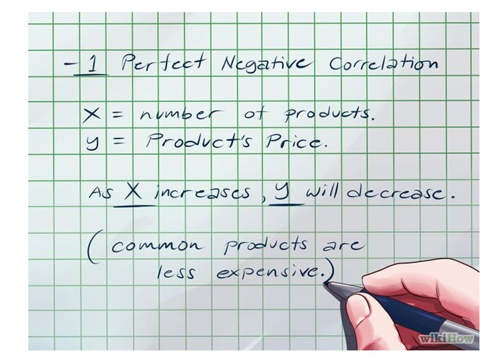
26. Know that a correlation of -1 indicates perfect negative correlation.
If your correlation is -1, this means that your variables are perfectly negatively correlated.
In other words, an increase in one will cause a decrease in the other, and vice versa.
As above, this relationship is linear. The rate at which the two variables grow apart from each other doesn't decrease with time.
As an example of this sort of correlation, let's consider a very basic supply and demand scenario. In extremely simplified terms, if x equals the number of products a company makes and y equals the price it charges for these products, as x increases, y will decrease. In other words, the more common a product becomes, the less expensive it becomes.

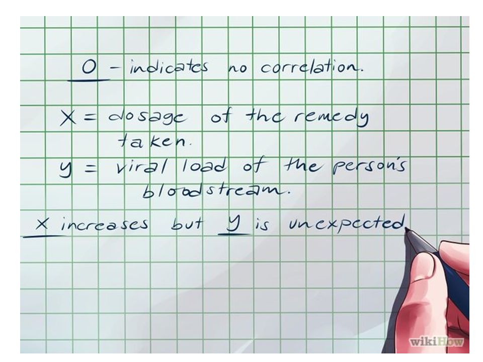
28. Know that a correlation of 0 indicates no correlation.
If your correlation is equal to zero, this means that there is no correlation at all between your variables.
In other words, an increase or decrease in one will not necessarily cause an increase or decrease in the other with any predictability.
There is no linear relationship between the two variables, but there might still be a non-linear relationship.
As an example of this sort of correlation, let's consider the case of someone who is taking a homeopathic remedy for a viral illness. If x represents the dosage of the remedy taken and y represents the viral load in the person's bloodstream, we wouldn't necessarily expect y to increase or decrease as x increases. Rather, any fluctuation in y would be completely independent of x.

30. Know that another value between -1 and 1 indicates imperfect correlation.
Most correlation values aren't exactly 1, -1, or 0.
Usually, they are somewhere in between. Based on how close a given correlation value is to one of these benchmarks, you can say that it is more or less positively correlated or negatively correlated.
For example, a covariance of 0.8 indicates that there is a high degree of positive correlation between the two variables, though not perfect correlation. In other words, as x increases, y will generally increase, and as x decreases, y will generally decrease, though this may not be universally true.

32. An Example

33. Do everything this time using matrices
Data
Means
Deviations
Covariance
Matrix ??

34. Covariance Matrix
We can interpret the variance and covariance statistics in matrix V to understand how the various test scores vary and covary.
Shown in red along the diagonal, we see the variance of scores for each test. The art test has the biggest variance (720); and the English test, the smallest (360). So we can say that art test scores are more variable than English test scores.
The covariance is displayed in black in the off-diagonal elements of matrix V.
The covariance between math and English is positive (360), and the covariance between math and art is positive (180). This means the scores tend to covary in a positive way. As scores on math go up, scores on art and English also tend to go up; and vice versa.
The covariance between English and art, however, is zero. This means there tends to be no predictable relationship between the movement of English and art scores.

35. How to use Covariance of Features
Can we use this valuable covariance information among different features of our data for something valuable?

36. Principle Component Analysis
Finds the principle components of the data

37. Projection onto Y axis
The data isn’t very spread out here, therefore it doesn’t have a large variance. It is probably not the principal component.

38. Projection onto X axis
On this line the data is way more spread out, it has a large variance.

39. Eigenvectors and Eigenvalues in PCA
When we get a set of data points, we can deconstruct the set’s covariance matrix into eigenvectors and eigenvalues.
Eigenvectors and values exist in pairs: every eigenvector has a corresponding eigenvalue.
An eigenvector is a direction, in the example above the eigenvector was the direction of the line (vertical, horizontal, 45 degrees etc.)
An eigenvalue is a number, telling you how much variance there is in the data in that direction, in the example above the eigenvalue is a number telling us how spread out the data is on the line.
The eigenvector with the highest eigenvalue is therefore the principal component.

40. Example

41. Example: 1st Principle Component

42. Example: 2nd Principle Component

44. Dimensionality Reduction

45. Only 2 dimensions are enough
ev3 is the third eigenvector, which has an eigenvalue of zero.

46. Reduce from 3D to 2D

47. How to select the reduced dimension?
Can I automatically select the number of effective dimensions of my data?
What is the extra information that I need to specify for doing this automatically?
Does PCA consider your data’s labels?