1. EE663 Image Processing Histogram Equalization Dr. Samir H. Abdul-Jauwad Electrical Engineering Department King Fahd University of Petroleum & Minerals

2. Image Enhancement: Histogram Based Methods  The histogram of a digital image with gray values is the discrete function n k : Number of pixels with gray value r k n: total Number of pixels in the image  The function p(r k ) represents the fraction of the total number of pixels with gray value r k. What is the histogram of a digital image?

3.  Histogram provides a global description of the appearance of the image.  If we consider the gray values in the image as realizations of a random variable R, with some probability density, histogram provides an approximation to this probability density. In other words,

4. Some Typical Histograms  The shape of a histogram provides useful information for contrast enhancement. Dark image

5. Bright image Low contrast image

6. High contrast image

7. Histogram Equalization  Let us assume for the moment that the input image to be enhanced has continuous gray values, with r = 0 representing black and r = 1 representing white.  We need to design a gray value transformation s = T(r), based on the histogram of the input image, which will enhance the image.  What is the histogram equalization?  he histogram equalization is an approach to enhance a given image. The approach is to design a transformation T(.) such that the gray values in the output is uniformly distributed in [0, 1].

8.  As before, we assume that: (1) T(r) is a monotonically increasing function for 0  r  1 (preserves order from black to white). (2) T(r) maps [0,1] into [0,1] (preserves the range of allowed Gray values).

9.  Let us denote the inverse transformation by r  T -1 (s). We assume that the inverse transformation also satisfies the above two conditions.  We consider the gray values in the input image and output image as random variables in the interval [0, 1].  Let p in (r) and p out (s) denote the probability density of the Gray values in the input and output images.

10.  If p in (r) and T(r) are known, and r  T -1 (s) satisfies condition 1, we can write (result from probability theory):  One way to enhance the image is to design a transformation T(.) such that the gray values in the output is uniformly distributed in [0, 1], i.e. p out (s)  1, 0  s  1  In terms of histograms, the output image will have all gray values in “equal proportion”.  This technique is called histogram equalization.

11.  Consider the transformation  Note that this is the cumulative distribution function (CDF) of p in (r) and satisfies the previous two conditions.  From the previous equation and using the fundamental theorem of calculus, Next we derive the gray values in the output is uniformly distributed in [0, 1].

12.  Therefore, the output histogram is given by  The output probability density function is uniform, regardless of the input.  Thus, using a transformation function equal to the CDF of input gray values r, we can obtain an image with uniform gray values.  This usually results in an enhanced image, with an increase in the dynamic range of pixel values.

13.  Step 1:For images with discrete gray values, compute: L: Total number of gray levels n k : Number of pixels with gray value r k n: Total number of pixels in the image Step 2: Based on CDF, compute the discrete version of the previous transformation : How to implement histogram equalization?

14. Example:  Consider an 8-level 64 x 64 image with gray values (0, 1, …, 7). The normalized gray values are (0, 1/7, 2/7, …, 1). The normalized histogram is given below: NB: The gray values in output are also (0, 1/7, 2/7, …, 1).

15. Gray value # pixels Normalized gray value Fraction of # pixels

16.  Applying the transformation, we have

17.  Notice that there are only five distinct gray levels --- (1/7, 3/7, 5/7, 6/7, 1) in the output image. We will relabel them as (s 0, s 1, …, s 4 ).  With this transformation, the output image will have histogram

18. Histogram of output image # pixels Gray values  Note that the histogram of output image is only approximately, and not exactly, uniform. This should not be surprising, since there is no result that claims uniformity in the discrete case.

19. Example Original image and its histogram

20. Histogram equalized image and its histogram

21.  Comments: Histogram equalization may not always produce desirable results, particularly if the given histogram is very narrow. It can produce false edges and regions. It can also increase image “graininess” and “patchiness.”

23. Histogram Specification (Histogram Matching)  Histogram equalization yields an image whose pixels are (in theory) uniformly distributed among all gray levels.  Sometimes, this may not be desirable. Instead, we may want a transformation that yields an output image with a pre-specified histogram. This technique is called histogram specification.

24.  Given Information (1) Input image from which we can compute its histogram. (2) Desired histogram.  Goal Derive a point operation, H(r), that maps the input image into an output image that has the user-specified histogram.  Again, we will assume, for the moment, continuous-gray values.

25. Input image Uniform image Output image s=T(r)v=G(z) z=H(r) Approach of derivation = G -1 (v=s=T(r))

26.  Suppose, the input image has probability density in p(r). We want to find a transformation z  H (r) , such that the probability density of the new image obtained by this transformation is p out (z), which is not necessarily uniform. This gives an image with a uniform probability density.  First apply the transformation  If the desired output image were available, then the following transformation would generate an image with uniform density: (**) (*)

27.  From the gray values  we can obtain the gray values z by using the inverse transformation,  z  G -1 (v) will generate an image with the specified density out p(z), from an input image with density in p(r) !  If instead of using the gray values  obtained from (**), we use the gray values s obtained from (*) above (both are uniformly distributed ! ), then the point transformation Z=H(r)= G -1 [ v=s =T(r)]

28.  For discrete gray levels, we have  If the transformation z k  G(z k )  is one-to-one, the inverse transformation s k  G -1 (s k ) , can be easily determined, since we are dealing with a small set of discrete gray values.  In practice, this is not usually the case (i.e., ) z k  G(z k )  is not one-to-one) and we assign gray values to match the given histogram, as closely as possible.

29. Algorithm for histogram specification: (1) Equalize input image to get an image with uniform gray values, using the discrete equation: (2) Based on desired histogram to get an image with uniform gray values, using the discrete equation: (3) )]([ )( 11 rTGz v=s Gz  

30. Example:  Consider an 8-level 64 x 64 previous image. Gray value # pixels

31.  It is desired to transform this image into a new image, using a transformation Z=H(r)= G -1 [T(r)], with histogram as specified below: Gray values # pixels

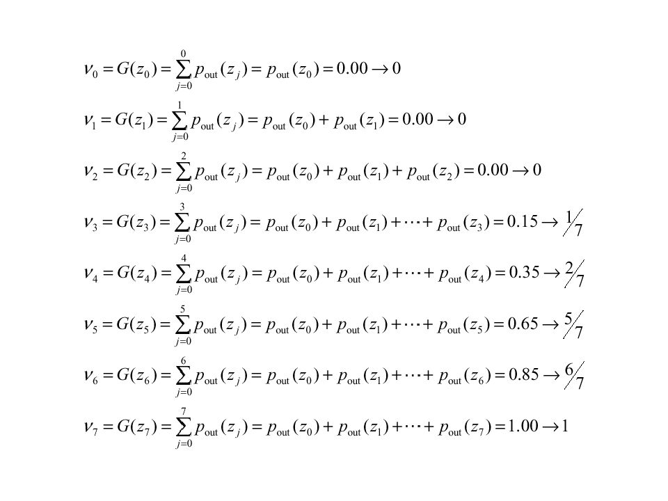
32.  The transformation T(r) was obtained earlier (reproduced below):  Now we compute the transformation G as before.

34.  Computer z=G -1 (s)  Notice that G is not invertible. G -1 (0) = ? G -1 (1/7) = 3/7 G -1 (2/7) = 4/7 G -1 (4/7) = ? G -1 (5/7) = 5/7 G -1 (6/7) = 6/7 G -1 (1) = 1 G -1 (3/7) = ?

35.  Combining the two transformation T and G -1, compute z=H(r)= G -1 [v=s=T(r)]

36.  Applying the transformation H to the original image yields an image with histogram as below:  Again, the actual histogram of the output image does not exactly but only approximately matches with the specified histogram. This is because we are dealing with discrete histograms.

37. Original image and its histogram Histogram specified image and its histogram

38. Desired histogram