Download presentation
Presentation is loading. Please wait.

1
Part III The General Linear Model Chapter 9 Regression

3
GLM, applied to regression Example 9.3.1 from Snedecor and Cochran (1989) Interested in the relationship between: – phosphorus content of corn (Pcorn in ppm) & phosphorus levels in soil samples (Psoil in ppm).
 Interested in the relationship between: – phosphorus content of corn (Pcorn in ppm) & phosphorus levels in soil samples (Psoil in ppm).")
4
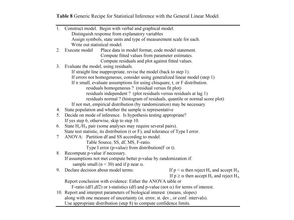
1. Construct Model Verbal Graphical Formal

5
1. Construct Model NameUnitsDimensionsMeasurement Scale Response Explanatory Graphical Verbal Phosphorus content of corn (Pcorn) depends on Phosphorus content of soil (Psoil)
 depends on Phosphorus content of soil (Psoil).")
6
1. Construct Model Verbal Graphical Formal Phosphorus content of corn (Pcorn) depends on Phosphorus content of soil (Psoil) UnitsDimensionsMeasurement Scale
 depends on Phosphorus content of soil (Psoil) UnitsDimensionsMeasurement Scale.")
7
2. Execute analysis. Place data in model format: lm1 <- lm(Pcorn~Psoil, data=corn) 2. Execute analysis. Compute fitted values and residuals. fits <- fitted(lm1) resid <- residuals(lm1) cbind(corn, fits, resid)
 resid <- residuals(lm1) cbind(corn, fits, resid).")
8
3. Evaluate Model. Plot residuals against fitted values Check linear trend

9
3. Evaluate Model. Plot residuals against fitted values plot(fits,resid,pch=16) Check linear trend
 Check linear trend")
10
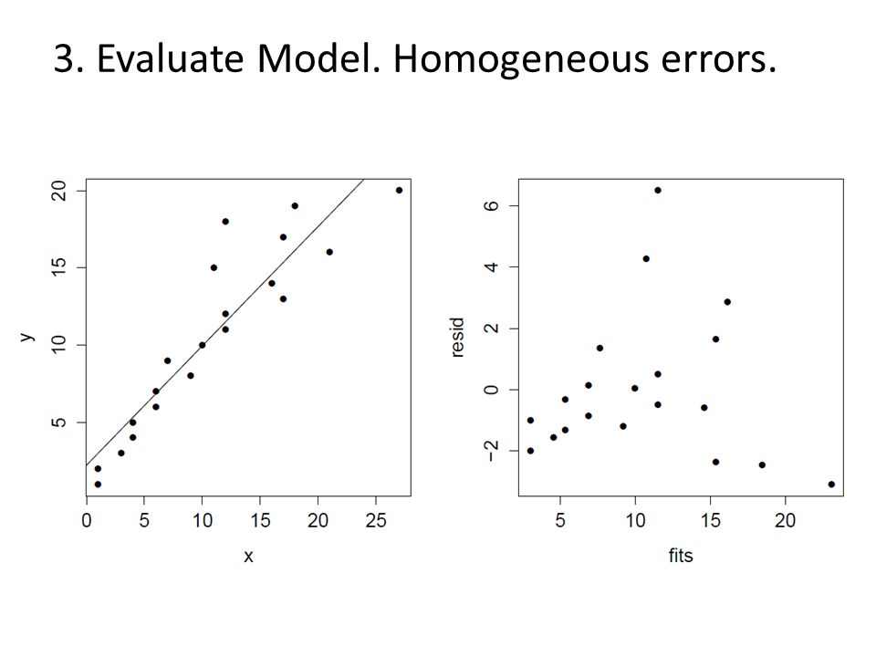
3. Evaluate Model. Plot residuals against fitted values

11
3. Evaluate Model. Using theoretical distributions ( χ 2, t, F) to calculate p-value, therefore we need to check their assumptions: – Fixed variance (errors homogeneous) – Normally distributed errors. – Independent errors – Unbiased estimate (errors sum to zero)
 to calculate p-value, therefore we need to check their assumptions: – Fixed variance (errors homogeneous) – Normally distributed errors. – Independent errors – Unbiased estimate (errors sum to zero).")
12
3. Evaluate Model. Homogeneous errors.

14
3. Evaluate Model. Normal errors.

15
3. Evaluate Model. Independent errors. This is a text example, we do not have information on spatial layout of samples, or on collection sequence. We will assume independence 3. Evaluate Model. Conclusion. Residuals appear to homogeneous, but not normal. We assume independence, we do not have enough information to evaluate this assumption. We may need to use an empirical distribution to compute p- values or confidence limits

16
4. State population and whether sample is representative. Population? Sample (n=9) The population is all values of phosphorus in corn, given knowledge of phosphorus in the soil The sample is representative if the 17 soil types represent the range of possible soil types
 The population is all values of phosphorus in corn, given knowledge of phosphorus in the soil The sample is representative if the 17 soil types represent the range of possible soil types.")
17
5. Decide on mode of inference. Is hypothesis testing appropriate? Since the relationship between P and P content in corn is unknown, we proceed 6. State H A / H o, test statistic and α HA:HA: Ho:Ho: Statistic:α:

18
7. ANOVA: partition df according to model. n=9 df tot = ________ = _____ df model = 1 df res = df total – df model = _____

19
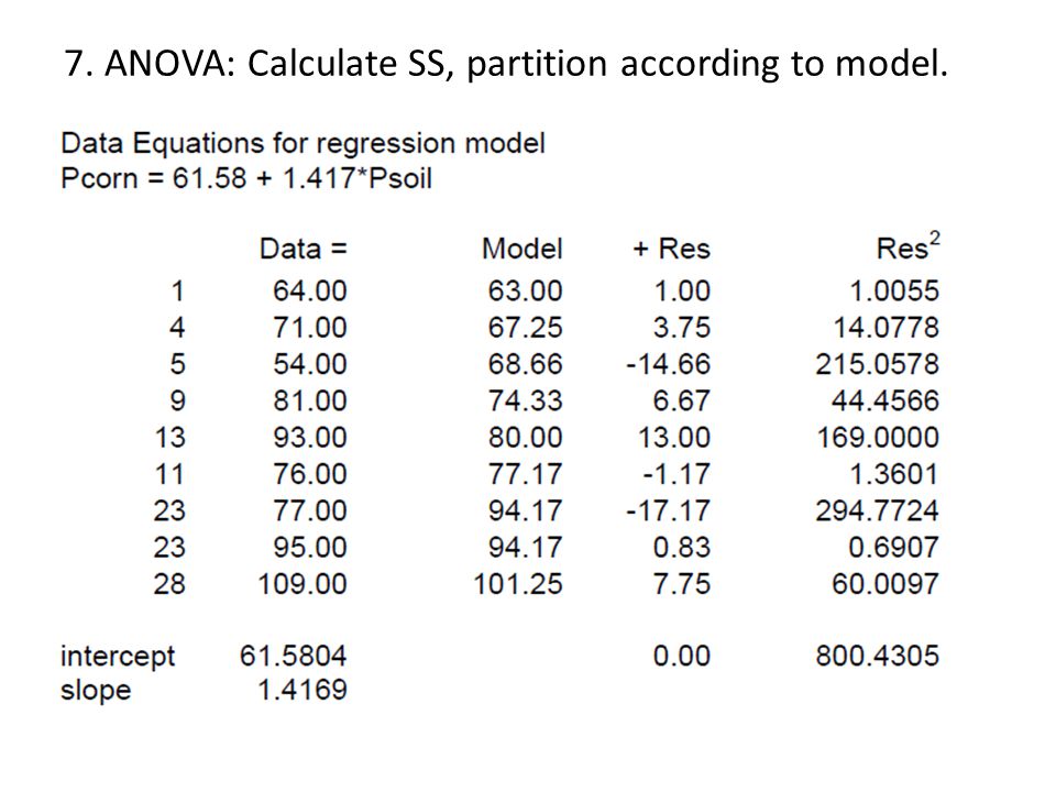
7. ANOVA: Calculate SS, partition according to model.

21
Null model: Pcorn = mean(Pcorn) SS total: 2274.00 Regression model: 61.58 + 1.417*Psoil SS residual: 800.43 SS improvement? __________

22
7. ANOVA: Calculate SS, partition according to model.

23
7. ANOVA: Partition df, SS according to model. Complete ANOVA table 7. ANOVA: Calculate Type I error from F distribution. Packages compute and place the p-value in the ANOVA table p = 0.00885

24
8. Recompute p-value if necessary. p-values can be inaccurate if assumptions are violated Distortion depends on sample size – As a rule of thumb, distortion is greatest if n < 30 – less serious if 30 < n < 100 – usually not serious if n > 100 When assumptions are not met, recompute Type I error if two conditions are met: 1.n small 2.p near α

25
8. Recompute p-value if necessary. Due diligence recompute p-value using randomization – Free of assumptions In 4000 randomizations there were 27 instances of an F-ratio greater than 12.89 – Empirical p-value: 0.00675 – Theoretical p-value:0.008854

26
9. Declare and report decision about model terms.

27
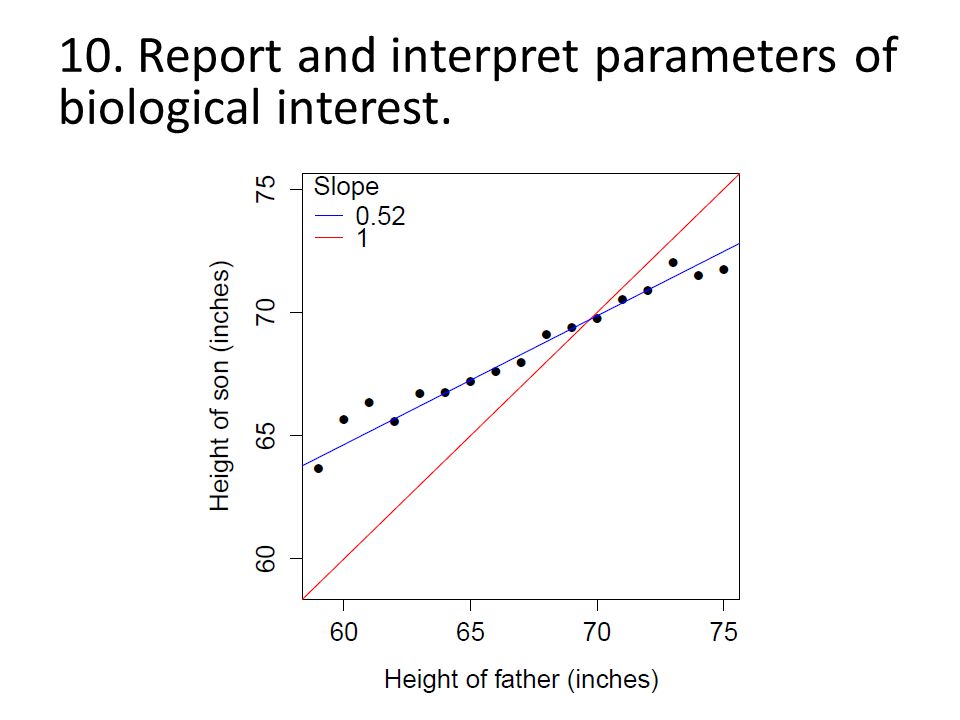
10. Report and interpret parameters of biological interest.

28
Today: Lab 4 due Monday & Tuesday: No classes Wednesday: Grad seminar Lecture Quizz 5 Thursday: Lab 5a

29
Chapter 9.2 Regression. Explanatory Variable Fixed into Classes

30
GLM, applied to regression X variable fixed into classes Example: Galton’s Law Quantity of interest is the stature (height) of sons in relation to stature (height) of their fathers. Data collected by Francis Galton at end of the 19th century. 1 st application of regression

31
1. Construct Model Verbal Graphical Formal Data

32
1. Construct Model Verbal Graphical Formal Data There is a positive relation between heights of sons and fathers Explanatory: _____________ Response:_____________ Model: __________________

33
1. Construct Model SymbolUnitsDimensionsMeasurement Scale H son HfHf ………

34
2. Execute analysis. Place data in model format: lm1 <- lm(Hson~Hf, weights=Nfamily, data=Heights) ………
 ……….")
35
2. Execute analysis. Compute fitted values and residuals. coefficients(lm1) (Intercept) Hf 33.2855960 0.5225171 63.667=+ 65.643=+ ………
 (Intercept) Hf = =+ ……….")
36
3. Evaluate Model □ Straight line model ok? □ Errors homogeneous? □ Errors normal? □ Errors independent?

37
4. State population and whether sample is representative. Population is all possible measurements, given the measurement protocol, if we repeated the study thousands of times We infer a population consisting of thousands of runs of the same experiment, using the same protocol

38
5. Decide on mode of inference. Is hypothesis testing appropriate? Might expect a 1:1 ratio Undertake hypothesis testing? Use confidence limits 10. Report and interpret parameters of biological interest. Compute confidence limits from standard error of the slope parameter summary(lm1)$coefficients Coefficients: Estimate Std. Error t value Pr(>|t|) (Intercept) 33.28560 1.64243 20.27 2.61e-12 *** Hf 0.52252 0.02424 21.55 1.06e-12 ***
$coefficients Coefficients: Estimate Std. Error t value Pr(>|t|) (Intercept) e-12 *** Hf e-12 ***.")
39
10. Report and interpret parameters of biological interest.

43
Chapter 9.3 Regression. Explanatory Variable Measured with Error

44
Adds bias to regression parameter estimates Example: – Relation between number of eggs and body size in cabezon fish (Box 14.12, Sokal and Rohlf 1995) – What is the magnitude of the bias? GLM, applied to regression Explanatory Variable Measured with Error

45
1. Construct Model Verbal – Does egg number N eggs depend on body mass M ? Graphical D V G F Formal – Response: N eggs – Explanatory: M units? dimensions? measurement scale?

46
2. Execute analysis. Place data in model format: lm1 <- lm(Neggs~M, data=data) Estimate parameters and compute fitted values and residuals
 Estimate parameters and compute fitted values and residuals.")
47
2. Execute analysis. Place data in model format: lm1 <- lm(Neggs~M, data=data) Estimate parameters and compute fitted values and residuals
 Estimate parameters and compute fitted values and residuals.")
48
3. Evaluate Model □ Structure? □ Straight line model ok? □ Errors homogeneous? □ Errors normal? □ Errors independent?

49
3. Evaluate Model □ Structure? □ Straight line model ok? □ Errors homogeneous? □ Errors normal? □ Errors independent?

50
3. Evaluate Model □ Structure? □ Straight line model ok? □ Errors homogeneous? □ Errors normal? □ Errors independent? M Neggs Res Lag.Res 14 61 15.05 NA 17 37 -14.56 15.05 24 65 0.35 -14.56 25 69 2.48 0.35 27 54 -16.26 2.48 33 93 11.52 -16.26 34 87 3.65 11.52 37 89 0.04 3.65 40 100 5.43 0.04 41 90 -6.43 5.43 42 97 -1.30 -6.43

51
4. State population and whether sample is representative. a)All measurements that could have been made on the fish by this protocol b)All cabezon fish c)All fish that could have been collected when the collection was made d)Measurements from 11 cabenzon fish reported here
All measurements that could have been made on the fish by this protocol b)All cabezon fish c)All fish that could have been collected when the collection was made d)Measurements from 11 cabenzon fish reported here.")
52
5. Decide on mode of inference. Is hypothesis testing appropriate? We want to know if the relationship between body size and egg count deviates from 1:1 Use confidence limits 10. Report and interpret parameters of biological interest. Compute confidence limits confint(lm1) 2.5 % 97.5 % (Intercept) -4.098376 43.632008 M 1.117797 2.622113
 2.5 % 97.5 % (Intercept) M")
53
10. Report and interpret parameters of biological interest. Neggs=Fits+Res 61=45.95+15.05 37=51.56+-14.56 65=64.65+0.35 69=66.52+2.48 54=70.26+-16.26 93=81.48+11.52 87=83.35+3.65 89=88.96+0.04 100=94.57+5.43 90=96.43+-6.43 97=98.30+-1.30 Check limits free of assumptions – randomization 3.65 2.48 -14.56 0.04 15.05 -1.30 5.43 -6.43 0.35 -16.26 11.52 49.60 54.04 50.09 66.56 85.31 80.17 88.78 82.52 94.92 80.18 109.83

54
10. Report and interpret parameters of biological interest.

56
Chapter 9.4 Exponential Function, using Linear Regression

57
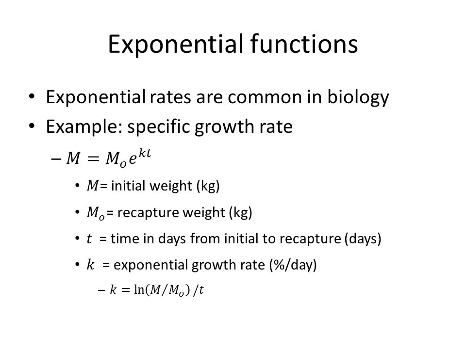
Exponential functions

59
Exponential rates are common in biology Example: specific growth rate – Growth of 6 lungfish in 2001 in Lake Baringo, Kenya kg kg Time Initial End Days 1.32 1.46 50 1.30 1.48 64 1.60 1.84 65 0.76 0.90 56 0.60 0.65 20 2.74 2.86 48

60
1. Construct Model Verbal – Growth rate of lungfish is exponential, with fixed growth rate k Graphical D V G F

61
2. Execute analysis.

62
3. Evaluate Model □ Straight line model ok? □ Errors homogeneous? □ Errors normal? □ Errors independent?

63
4. State population and whether sample is representative. All measurements that could have been made on the fish by this protocol 5. Decide whether to use hypothesis testing. The research objective is to estimate specific growth rate of fish. We will examine the parameters and compute confidence limits (skip to step 10).
..")
64
10. Report and interpret parameters of biological interest. Compute confidence limits Limits bound zero, suggesting no growth. Yet all fish were larger upon recapture. Improbable result: – 0.5 6 = 0.0156 But was growth exponential? confint(lm1) 2.5 % 97.5 % (Intercept) -0.133723588 0.197839514 t -0.001595261 0.004696776 L = Lower limit = -0.160 %/day U = Upper limit = 0.470 %/day
 2.5 % 97.5 % (Intercept) t L = Lower limit = %/day U = Upper limit = %/day.")
65
10. Report and interpret parameters of biological interest. The estimate of growth rate is approximately 0.1%/day, or about 3% per month – but the estimate is not reliable!

Similar presentations

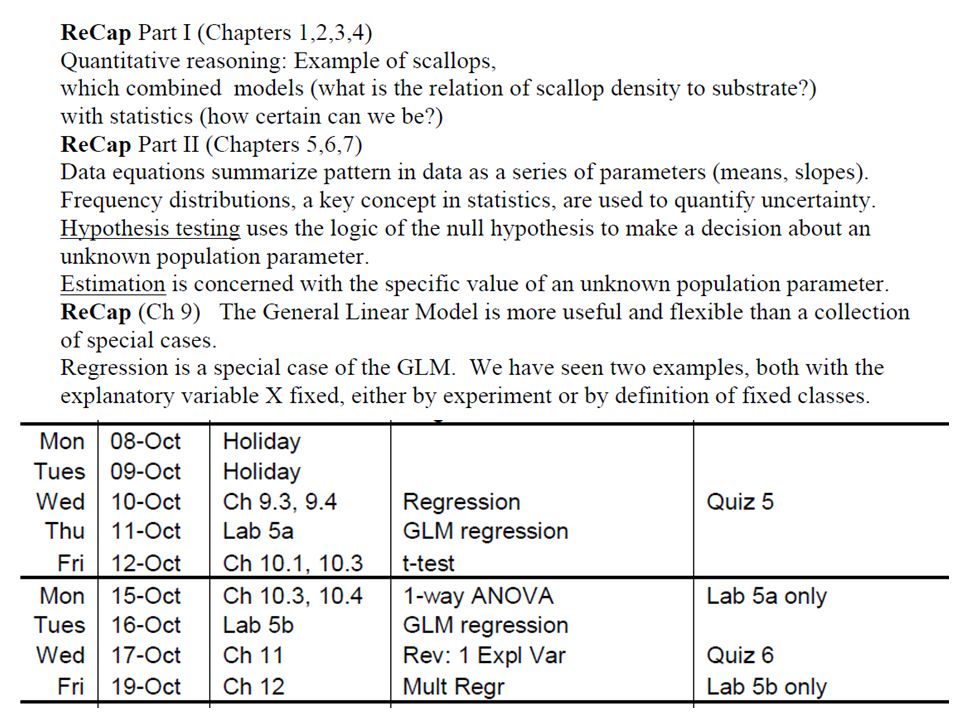


 GLM Review on Friday 2) Exam II on Monday.>")

>")


 Review>")


