1. Meteorology is: - Part Art - Part Science - Part Mythology As Science increases, so must Understanding Models provide Guidance, not Forecasts

2. The Data Collection Step Building a Numerical Weather Prediction System

3. Global Observing Systems

4. 1200 Z Global Rawinsondes

5. United States Radar Network

6. Northern Hemisphere Marine Observations -- 12 Hour Total

7. 1200Z Aircraft Wind/Temperature Reports

8. 0000Z North American Automated Aircraft Reports

9. Geostationary Satellite Cloud Tracked Winds

10. 1200Z Polar Satellite Temperature/Humidity Sounding Information

11. Microwave Precipitable Water/Temp/Moisture/Surface Winds

12. The Data Quality Control Step Building a Numerical Weather Prediction System

13. The Data Quality Control Process

14. Data Rejection List - Based on Individual Station History

15. Gross Error Checks - Based of Acceptable Data Thresholds

16. Complex Quality Control - Attempts to Correct Errors Neighbor Checks - Comparison with Nearby Values

17. Temporal Checks - Assure Consistency Over Time

18. Temporal Checks - Also Help Resolve Neighbor Checks

19. People Still Need to Correct the Most Difficult Problems

20. The Data Analysis Step Building a Numerical Weather Prediction System

21. The Analysis Problem - Depicting Data as Continuous Fields

22. Manual Analysis Produces Continuous Images

23. Objective Analyses InterpolateRandom Data to Regular Grids

24. Most Areal Weighting Procedures based on Distance and other factors

25. Basic Analysis Equation

26. We need Full Analysis Coverage, even over data sparse areas. NWP models move (advect) information from data rich into data sparse regions Why use a Background “First Guess” field? Can’t we Analyze the Data Directly?

27. Performing an Objective Analysis

28. The Analysis begins with a Earlier Forecast as “First Guess”

29. “First Guess” values are calculated at Observation Points

30. The Objective Analysis Uses Differences Calculated Between the Data and the First Guess - The Analysis “corrects” the First Guess

31. The Differences are Interpolated to the Regular Grid

32. Difference field shows errors in “First Guess Memory”, which the analysis then corrects. For the analysis to be effective, the errors should be small!

33. Combining the “First Guess” and Differences at Grid Points Yields the Final Grid Point Values Which shows changes beyond areas covered by Data

34. The Big Question becomes: How to determine the Optimal Analysis Analysis weights Older Optimal Interpolation schemes took into account: Station Proximity Observational Error Estimates “First Guess” Error Estimates Statistical/Dynamical Variable Correlation

35. Data Assimilation - What is it? In Data Sparse or Complex Areas, The Analysis is only as Good as The Guess To improve the Analysis First Guess, Need to include as much Data as possible into the Model at all times to be able to producing the Best First-Guess Possible for future analyses

36. Analyses without Data-Assimilation used longer-range forecast ‘First Guess” fields - 12 to 24 hour forecasts were often used -

37. Intermediate-time data were ignored and large corrections were made to the model “First-Guess” fields, creating imbalances

38. Data assimilation systems make a series of smaller changes to shorter-range “First-Guess” forecast fields

39. Use of 3-hourly analysis steps allows much more data to be used.

40. Forecasts using data assimilation based analyses preserve details in data better and require less time to become “dynamically active.”

41. Variational Analysis Techniques represented a major improvement in data assimilation. In the variational approach, analyses are made of the observed variables in their original form, rather than making all observations “look like” radiosonde data. For example, instead of analyzing temperature “soundings” determined from satellite radiances, the model “first guess” fields are converted to radiances and then the differences between the “first-guess” and observed radiances are analyzed and converted back to model forecast variables- This eliminates much “variable conversion error”

42. Variational Analysis represented a major improvement in data assimilation. An example of Previous Analysis Approachs: 1. Satellite radiances are observed over continuous areas (Area and Layer average data) 2. Representative “samples” are extracted to reduce data set size 3. Observations are “adjusted” to remove cloud contamination 4. Use radiative transfer laws are used to obtain layer-average temps. 5. Layer-averages are interpolated to standard rawinsonde levels 6. Model Guess is interpolated to sounding levels (x,y,z) 7. Differences are made between Guess and Satellite “data” 8. Differences Interpolated vertically to model levels 9. Differences Interpolated horizontall to grid to get continuous field

43. Variational Analysis represented a major improvement in data assimilation. Variational Approach: 1. Radiation laws used to convert temperatures and humidity data taken directly from the native vertical coordinate model to radiances in layers corresponding to satellite observations, including model cloud information 2. Model-based radiance are interpolated to all satellite observation locations 3. Difference between ‘First Guess” and observations calculated asin radiances 4. Radiance differences interpolated back to model grid along with all other data - including confidence in each data type 5. Radiation laws used to convert results back to temperature/humidity

44. Variational Analysis Techniques represented a major improvement in data assimilation. Although the computational techniques in variational analysis are much more complex than basic circular search procedures, the technique: 1. Eliminates much “variable conversion” error 2. Retains the maximum information from every data set 3. Allows a mixing of many “partial” observation - e.g., combine aircraft winds with 88-D radial velocity component 4. Is no more expensive to run 5. Improves forecast skill notably

45. This approach is still not the complete answer Although Data Assimilation systems have Improved the “First Guess’ Fields used for Analyses, the “Direction” of the “First Guess” forecast does not usually fit the data at intermediate times as well as it could Correction to “First Guess”

46. Continuous Assimilation (called 4-D Variational Analysis) Allows the analysis to create the best possible fit to the total set of observations throughout the entire assimilation period and their changes throughout the entire analysis period by repeatedly running the model both forward and backward – effectively making correction to many “First Guess” fields. The technique, however, needs many more computer resources Correction to “Initial” “First Guess” Correction to “Second” “First Guess”

47. The Forecast Model Building a Numerical Weather Prediction System

48. Forecast Models have 2 Essential Computational Components The Model Dynamics -- The Equations of Motion The Model Physics -- Physically forced Processes Many occur at small scales and must have their effects approximated

49. The Model Dynamics Equations of Motion determine how parcels of air move in response to accelerations produced by imbalances between atmospheric forces-Coriolis,Pressure Gradient...

50. Solar Heating in the tropics forces the Global General Circulation by creating pressure gradient forces

51. Equations of Motion in Simplest Form -- [Horizontal Winds] Parcel Acceleration (total derivative) = Sum of Coriolis and Pressure Gradient Forces However, because NWP forecasts are made at Points, not for Parcels

52. Therefore, Equations need to be written in terms of Local Wind Changes These are the Wind Prediction Equations Note the addition of ‘non-linear’ terms: - Changes in the u wind component are dependent both on the u wind itself and gradients of the u and v winds, - Likewise for the v wind component This can lead to numerical instability in grid point models if time computer time steps are too long – needs accurate gradient calculations

53. For Hydrostatic models, we also must assure Hydrostatic Balance and Mass Continuity [Continuity used to diagnose Vertical Motion] Finally, we add Heat and Moisture Conservation -- [Temperature and Moisture] The Combination of these 6 equations is the basis for all Hydrostatic Weather Prediction Models

54. Forecasts are produced by solving these Differential Equations using relatively simple arithmetic approximations to forecast Winds, Temperature, Humidity and Pressure U Future = U Now + Acceleration * Time Step

55. Models really forecasting for “Boxes” of Air

56. The Forecast “Box” size depends on the forecast Grid size

57. Regional Model Grids can be finer than Global Grids and Boundary Conditions from Global Models

58. Grid resolution limits the types Phenomena that can be forecasted since a minimum of 5-9 grids points are needed to define and retain a feature (wave) in the forecast

59. Most Operational Models use Terrain Following (Sigma) Vertical Coordinate Systems

60. Most Global Models use “spectral” instead of “grid” for Dynamics Formulations to increase resolution and save time But, Spectral Models still calculate “physics” on grids

61. In Spectral Models, Atmospheric waves divided into many wave components and forecast are made for each wave. Limits truncation errors because derivatives are known precisely (Derivative of Sine is Cosine, etc)

62. High-Resolution Non-Hydrostatic Models include much more realism - especially for Convectively Driven Phenomena - by including vertical as well as horizontal accelerations But at a high cost in Model Complexity and required resolution

63. Forecast Models have 2 Essential Computational Components The Model Dynamics -- The Equations of Motion -- Models do this part quite well - - - - - - - - - - - - - The Model Physics -- Physically forced Processes Many occur at small scales and must have their effects approximated

64. The Model Physics The Physics Part of Forecast Models approximates the Effects of major complex Physical Processes occuring in the atmosphere - often at smaller scales than can be modeled directly, for example Radiation, Precipitation, Turbulent Mixing, Friction,...

65. Radiation Parameterizations Simplified solutions to the full radiative transfer process. Often calculated in models over several time steps. Highly interactive with other model conditions - namely: Cloudiness Soil condition Vegetation Snow cover

66. Accurate Radiation requires detailed boundary layer information

67. How does this affect a sounding forecast? * Surface temperature change depends on incoming sunlight, surface conditions, advection, low-level lapse rate. * Incoming short-wave radiation (sunlight) affected by “cloudiness” in model, determined either from mean relative humidity or average liquid water content in 3-5 layers of the atmosphere. * Vertical mixing of temperature, moisture and momentum (winds) affected by surface temperature, boundary layer lapse rate and boundary layer wind shear - often based on combination of theoretical rules and observational studies.

68. Compound effects of radiation apparent in forecast soundings

69. By 9:00 AM Local, Surface is heating - Wind increasing

70. By Local Noon, Boundary Layer well mixed

71. By mid-afternoon, Momemtum mixes downward, transporting momentum and producing surface wind “gusts”

72. By Evening, Cooling separates Surface from Boundary Layer

73. On a clear, dry evening, the problem is simply one of calculating the temperature change due to outgoing longwave radiation, which itself depends on the surface temperature

74. When a layer of the atmosphere is humid or partly cloudy, only part of the longwave radiation goes directly to space, the remainder is absorbed and re-emitted to space and earth, usually at a lower rate

75. When the sky is cloud-covered, all of the longwave radiation is absorbed by the clouds and retransmitted upward and downward. Radiation is a very long computational process.

76. On a clear day, solar energy is partially reflected back to space and partially absorbed by the earth’s surface. The surface then re-radiates some longwave radiation to space and conducts other to the soil below and air above - part of which may be convected (mixed) to higher levels.

77. If the earth’s surface is dark or bare soil, less sunlight is reflected and more absorbed, which heats both the soil and the air more through conduction and convection.

78. If the surface is light colored, more solar radiation is reflected and less soil and atmospheric heating is predicted. For this to be predicted well, the model must have proper information on soil type.

79. As the cloud layer thickens, more solar radiation is reflected. For this to be predicted properly, the cloud layers must be relatively thick.

80. Snow is a very good reflector, especially at low sun angles. It also acts as a good insulator, reducing conduction of heat to/from the soil and long-wave radiation. Because little solar radiation is absorbed, atmospheric heating is low. Good snow-cover data is critical.

81. The amount of reflected sunlight also varies with time of day over oceans. Here, however, the radiation that is absorbed by the oceans surface is transported both upwards and downwards by convection in the atmosphere and the oceans.

82. If a lower atmospheric layers are moist, some of the incoming solar radiation will be scattered upward and downward, reducing the net incoming radiation and surface heating. Likewise, outgoing longwave radiation will be absorbed and retransmitted upward and downward.

83. Over dry soil, most of the solar radiation heats the soil, which in turn heats the lowest part of the atmosphere. This heat is then mixed upwards to heat successively deeper parts of the boundary layer. Heat also goes into the soil layers (another parameterized process)

84. Where the soil is moist, the solar radiation both heats and moistens the boundary layer, with evaporation reducing surface heating. Incorrect surface moisture in forecast models can cause local temperature and precipitation errors - depending on the area and degree of soil saturation

85. Most models also include information about vegetation type and seasonal growth rate. In areas of active plant growth, radiation is absorbed by the plants. Part is assumed to support the plant growth, while the remainder heats and moistens the boundary layer.

86. Soil models allow plants to move water from below the earth’s surface to the atmosphere through the process of evapo-transporation. This requires information about plant type and growth rate, soil type and past precipitation,....

87. What effect can this have on NWP Guidance? An extreme example of Improper Snow Cover Specification

88. Correct Snow Cover Analysis

89. Incorrect Snow Cover Analysis

90. Surface Temperature forecast with Incorrect Snow cover - Snow and Freezing Rain forecast along US East Coast

91. Surface Temperature forecast with Correct Snow Cover All Precipitation along US East Coast was forecast as rain

92. Forecast with Incorrect Snow cover was for Snow and Freezing Rain forecast along US East Coast Boundary Layer Temperature Errors exceeded 6C

93. Warning: The effects of Physical Parameterizations can produce misleadingly detailed dynamical responses, due to horizontal models resolution limits Inland extent of Sea Breeze depends on model grid spacing

94. Realism of Precipitation and its effects limited by grid resolution - and represent areal averages

95. NWP Models must be able to simulate many different types of clouds and precipitation

96. Precipitation Parameterization u Precipitation divided into two types in model: u “Large Scale” or “Grid Scale” Precipitation - Which is used to simulate the occurance of Stratiform Precipitation u “Convective” - which is used to account for the effects of deep convection on heating and moistening the atmosphere u Not having a separation allows too much latent heating to concentrate at low levels in the atmosphere and produce overdevelopment.

97. “Grid Scale” Precipitation The Forecast models essentially emulate what you, as forecasters, do using a thermodynamic diagram. Air is lifted by the vertical motions predicted in the model. When a Relative Humidity saturation limit is reached (usually between 90-98%), precipitation forms. It falls to the ground, with some evaporating and moistening the lower model layers. The Forecast models essentially emulate what you, as forecasters, do using a thermodynamic diagram. Air is lifted by the vertical motions predicted in the model. When a Relative Humidity saturation limit is reached (usually between 90-98%), precipitation forms. It falls to the ground, with some evaporating and moistening the lower model layers. Some models today are beginning to forecast Liquid Cloud Water, in which case when saturation occurs, clouds are formed first, followed by precipitation.

98. - Grid-scale precipitation and cloud parameterization (PCP) are model emulations of cloud and precipitation processes that remove excess atmospheric moisture directly resulting from the dynamically driven forecast wind, temperature, and moisture fields. - While grid-scale motions determine the forcing, additional cloud and precipitation processes occurring at scales much smaller than a grid box also influence the true microphysical response and must be parameterized.

99. - Development of clouds and precipitation in the PCP scheme results in latent heating from condensation (indicated by the red area in the animation), which changes the wind, temperature, and moisture fields. - Evaporative cooling of the air from falling precipitation takes place in subsaturated layers below where precipitation is formed (the blue area in the animation). - Over time, these feedbacks onto model forecast variables may further strengthen the circulation that initially produced the model clouds and precipitation. The strengthened circulation may increase the precipitation and latent heating, which, in turn, may result in additional feedbacks.

100. Grid-scale precipitation and cloud parameterization (PCP) are model emulations of cloud and precipitation processes that remove excess atmospheric moisture directly resulting from the dynamically driven forecast wind, temperature, and moisture fields.

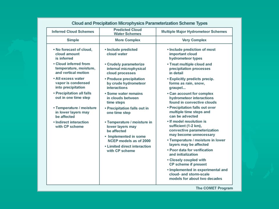
101. - Traditionally, PCP schemes had infer the presence of clouds in grid layers based upon RH saturation thresholds and immediately condense all excess moisture into precipitation. Most schemes originally used 100% RH as the critical RH saturation threshold, but later used values between 75% and 85% to account for scattered precipitation within grid box. - Recent advances in model horizontal/vertical resolution, physics, and computing power have allowed more realistic PCP schemes that include predicted cloud water. These schemes range from simple schemes that account for cloud water only to more complex schemes that include many types of hydrometeors and internal cloud processes.

102. - Despite the improved simulation of physical processes in PCP schemes, the model's large-scale forcing fields continue to play a larger role in determining the amount of precipitation over a broad region from a given weather system than the degree of detail in the PCP scheme

103. Using Inferred Clouds: Description, Models, & Process These schemes infer precipitation to remove excess moisture and infer clouds, all based on RH. (Note that this order is not physically correct, since precipitation forms from clouds in reality.) Process of removing grid-scale moisture: - Areas of excess moisture or supersaturation must be present in the sounding to diagnose precipitation, not including cloud ice or phase changes

104. Using Inferred Clouds: Description, Models, & Process -In areas of excess moisture or supersaturation, temperatures warm from latent heat release, and the specific humidity and dewpoint decrease as water vapor condenses until the temperature and dewpoint are equal -Precipitation falls out instantaneously. Sub-saturated areas beneath the precipitation production layers are cooled and moistened by the evaporation of some falling precipitation - All water in the atmosphere remains in vapor form. The resulting RH is too high, because no water is held in cloud

105. In contrast to schemes using inferred clouds, schemes using predicted clouds follow a physically based sequence of forming clouds prior to precipitation. Schemes using simple clouds diagnose precipitation from cloud water (or ice) only. Schemes using complex clouds, on the other hand, predict precipitation directly through the modeling of internal cloud processes, including multiple cloud and precipitation hydrometeor types.

106. Schemes Using Simple Clouds: Description, Models, & Process Description: These are schemes that predict cloud water/ice based on RH and then infer or diagnose precipitation based on cloud water/ice amount -Uses critical RH level (generally below 100%) to account for sub grid-scale moisture variability in order to account for the amount of cloud water -Supersaturation is not required to create cloud liquid and ice -Forms clouds first -Accounts for partial cloudiness through overcast cloud cover as RH increases above the critical value

107. Schemes Using Simple Clouds: Description, Models, & Process Description: These are schemes that predict cloud water/ice based on RH and then infer or diagnose precipitation based on cloud water/ice amount -Where cloud water is condensed, latent heat is released and specific humidity is reduced, warming the temperature and lowering the dewpoint and RH around the cloud -May include cloud ice and supercooled cloud droplets -In sub-freezing cloud layers, the cloud water phase may depend upon physical parameters, such as cloud top temperature -May crudely emulate interactions between supercooled cloud water and ice, thereby accounting for temperature effects on precipitation rates

108. Schemes Using Simple Clouds: Description, Models, & Process Description: These are schemes that predict cloud water/ice based on RH and then infer or diagnose precipitation based on cloud water/ice amount -If the cloud water amount exceeds a critical value, precipitation is created from cloud water -Precipitation may be produced within the cloud from a combination of cloud water creation, advection, and, in some more complete PCP schemes, input of diagnosed convective cloud water from the model's CP scheme

109. Schemes Using Simple Clouds: Description, Models, & Process Description: These are schemes that predict cloud water/ice based on RH and then infer or diagnose precipitation based on cloud water/ice amount -In areas of excess moisture or supersaturation, temperatures warm from latent heat release, and the specific humidity and dewpoint decrease as water vapor condenses until the temperature and dewpoint are equal -Precipitation falls out instantaneously. Sub-saturated areas beneath the precipitation production layers are cooled and moistened by the evaporation of some precipitation -The resulting RH is more realistic because some water and ice is condensed in clouds; not all is held in vapor form as in inferred cloud schemes

110. Schemes Using Simple Clouds - Strengths: -Measurable improvement in precipitation amount and location over schemes with inferred cloud because: -Clouds can be advected, -The effects of cloud ice on precipitation processes can be accounted for, which allows more realistic microphysics parameterization, - RH fields are more realistic since some water and/or ice is held in clouds -The PCP scheme may have direct interaction with the CP scheme through input of convective cloud water - Allow direct comparisons of model initial and forecast cloud fields with satellite imagery -Allow assimilation of cloud data to improve moisture fields since cloud water is a predicted variable -Allow direct and consistent linkage between cloud and radiation processes -Distinguishing between cloud water and ice improves the simulation of radiative effects of water versus ice clouds -- Are better suited for higher-resolution models because more microphysics details and smaller-scale motions can be taken into account

111. Schemes Using Simple Clouds – Limitations: -More computationally expensive -Improvements in precipitation forecast are not complete because : -Precipitation is still a byproduct, rather than predicted directly, and falls to the ground in one time step -Important microphysical parameterizations are relatively crude -Precipitation hydrometeors are not explicitly predicted, which affects forecast precipitation location and amount, especially for very light and heavy precipitation and where horizontal advection of precipitation is important (primarily snow) -The precipitation rate is an average for a grid box which can lead to: -Over or under forecasts of precipitation by the model depending upon the actual extent and rate of the precipitation -In reality, precipitation rates may vary considerably at individual points within a grid-box area -In reality, sub grid-scale variability in precipitation amount increases as the grid-box area increases -Microphysics are too simple to be able to predict convective processes, such as the creation of cold pools and gust fronts

112. Schemes Using Complex Clouds: Description, Models, & Process Description: These schemes predict clouds and precipitation based on RH by directly predicting precipitation hydrometeors and accounting for internal cloud processes. -These schemes are only used in higher-resolution models because they require sufficient model resolution to resolve small-scale variability affecting microphysical processes. -Use critical RH level (generally below 100%) to account for sub grid-scale moisture variability and patchy clouds -Supersaturation is not required to create cloud liquid and ice -Include multiple internal cloud processes, such as mixed phases and graupel

113. Schemes Using Complex Clouds: Description, Models, & Process Description: These schemes predict clouds and precipitation based on RH by directly predicting precipitation hydrometeors and accounting for internal cloud processes. -Where water vapor condenses onto any hydrometeor or becomes cloud liquid or ice, latent heat is released, warming the environmental temperature. -Water vapor is used in the condensation process, reducing the environmental specific humidity

114. Schemes Using Complex Clouds: Description, Models, & Process Description: These schemes predict clouds and precipitation based on RH by directly predicting precipitation hydrometeors and accounting for internal cloud processes. -As precipitation starts to fall from the cloud: -Cooling and moistening occur near the freezing level from melting and occur in the sub-cloud layer from evaporation -Mixed phase hydrometeor interactions and phase changes can occur

115. Schemes Using Complex Clouds: Description, Models, & Process Description: These schemes predict clouds and precipitation based on RH by directly predicting precipitation hydrometeors and accounting for internal cloud processes. -As precipitation falls from the cloud: -Precipitation is tracked as it falls to the ground, rather than falling to the ground instantaneously. -Sub-saturated areas moisten and cool as precipitation falls -Some water or ice remains held in clouds, making the resulting environmental RH more realistic

117. “Convective” Parameterizations Do not forecast Convection directly, but account for its effects. Necessary to transport latent heat and moisture into the upper troposphere - especially important in the tropics. Intensity and beginning usually related in some way to Moisture Flux Convergence. No scheme is perfect - Most “tuned” for tropical oceanic environments and all assume effects will occur over entire grid box. Remember: Convective Parameterizations are designed to STABILIZE the atmosphere, are ‘intermittent’, and do not match observed diurnal cycle in tropics

118. How Convection is Formed in a Model What happens when the PCP scheme tries to remove instability by creating "grid-scale" convection? The results depend largely upon how the scheme redistributes heat and moisture when it 'convects,' which, in turn, depends upon the types of motion that the dynamics in the model are able to forecast. Since model forecast vertical velocities are much smaller than actual convective updraft velocities, the moisture is carried upward too slowly and the PCP scheme releases latent heating over a longer period of time and primarily in the lower troposphere. -CP schemes parameterize the vigorous vertical transports done by updrafts and downdrafts, which move diabatically heated lower tropospheric air into the upper troposphere and evaporatively cooled mid- tropospheric air to the boundary layer. -Additionally, subsidence warming of the environment occurs below the convective cloud tops. A typical example of the net result looks like the blue curve in the graphic, with peak heating in the mid to upper levels.

119. Because cyclogenesis tends to occur in the layer where the heating rate increases rapidly with height, low-level cyclogenesis ensues if a model tries to create grid-scale convection with the PCP scheme. By contrast, when the CP scheme creates convection, the tendency toward cyclogenesis is at mid levels (for instance, like an MCC vortex) and is much weaker -Additionally, the low-level cyclogenesis occurring with PCP scheme grid-scale convection feeds back on itself by enhancing low-level convergence, which further intensifies the heating and cyclogenesis. -If the region of excessive latent heating and precipitation grows in size, the disturbance created can become dynamically balanced and long lasting, like a typical synoptic cyclone, although it may have warm core characteristics, especially in the lower troposphere. -Although this has sometimes been referred to as "convective feedback," the forecast errors result from what the CP scheme did not do!

120. Because cyclogenesis tends to occur in the layer where the heating rate increases rapidly with height, low-level cyclogenesis ensues if a model tries to create grid-scale convection with the PCP scheme. By contrast, when the CP scheme creates convection, the tendency toward cyclogenesis is at mid levels (for instance, like an MCC vortex) and is much weaker -Models use CP schemes to relieve instability before the PCP scheme tries to form grid-scale convection! -Note: If the CP scheme is used but fails to sufficiently relieve instability, the model will still make grid-scale convection where there is upward motion and sufficient moisture. -As model resolution increases, the area covered by a grid box decreases and the grid-scale vertical velocities increase, so the heating profile and consequent forecast impacts become more realistic. -When grid spacing gets down to 1 or 2 km, convection can be simulated directly and no CP scheme is used.

121. Role of CP in Models -In nature, convection not only produces precipitation, but also transport sheat upward, redistributes moisture, and thereby stabilizes the atmosphere. -If enough convection occurs over a large enough area, it can also create outflow jets and mid-level vortices and drive larger atmospheric circulations that affect weather in distant locations, etc.

122. Role of CP in Models To accomplish both tasks, each scheme must define the following, using information averaged over entire grid boxes: -What triggers convection in a grid column -How convection, when present, modifies the sounding in the grid column -How convection and grid-scale dynamics affect each other

123. Role of CP in Models -How a scheme handles these assumptions can limit its effectiveness. -Furthermore, the parameters used in the assumptions are adjusted to optimize the scheme's overall performance in all situations. -They may work well for some situations but work poorly for others. (They perform well in average situations but break down in extreme events.)

124. An example of the Kuo Scheme Description: A simple scheme produces precipitation and increases static stability by emulating moist-adiabatic ascent –temperature/moisture profiles  moist adiabatic Trigger: Convection is triggered by any pre-specified amount of Convective Available Potential Energy (CAPE) and column-integrated moisture convergence exceeding a threshold value

125. Kuo Scheme: Description, Models, & Trigger Description: A simple scheme produces precipitation and increases static stability by emulating moist-adiabatic ascent –temperature/moisture profiles  moist adiabatic -Moves temperature profile throughout the cloud toward a low-level moist adiabat. -Some of the moisture moistens the sounding while some falls instantly as rain.

126. Kuo Scheme: Description, Models, & Trigger Description: A simple scheme produces precipitation and increases static stability by emulating moist-adiabatic ascent –temperature/moisture profiles  moist adiabatic -The amount of rain produced varies by model, even for the same conditions. -The division of the moisture supply into that which moistens the sounding and the part that falls as rain can vary from model to model. -If most of the moisture is used for moistening the sounding, the PCP scheme may eventually generate some precipitation.

127. Kuo Scheme: Description, Models, & Trigger Description: A simple scheme produces precipitation and increases static stability by emulating moist-adiabatic ascent –temperature/moisture profiles  moist adiabatic -Link to large-scale forcing: The intensity and continuation of convective precipitation and sounding changes depend upon low-level moisture convergence -The scheme assumes that convection consumes moisture at the rate supplied by the large-scale wind and moisture fields.

128. Kuo Scheme: Description, Models, & Trigger Description: A simple scheme produces precipitation and increases static stability by emulating moist-adiabatic ascent –temperature/moisture profiles  moist adiabatic -Final state: Temperature and sub-saturated moisture profiles approach moist adiabatic, but do not reach them. -The scheme assumes that convection does not occupy the entire grid column, although it continues to moisten and approach moist adiabatic as convection persists.

129. Kuo Scheme: Strengths & Limitations Strengths: -Essence and behavior is easy to understand -Runs quickly; requires few computing resources Limitations: -Simplistic scheme; cannot represent the variety of things that happen in nature -Does not account for the strength of cap inhibiting convective development -Positive feedback (including precipitation bull's-eyes) sometimes occurs because the model response to parameterized convective heating may generate moisture convergence, which triggers the scheme again. This behavior stems from assuming that moisture convergence causes convection -Many variations exist (for example, some include downdrafts, while others do not). -Each formulation results in a variety of unrealistic physical behaviors

130. Many different Convective Parameterizations are used in various models Each scheme has it’s own advantages and disadvantages NONE of them simulate CONVECTION, only account for it’s effects Instead of spending all day talking about this, Much more information and examples are available in the online COMET NWP Training Module

131. Future Model Trends Future Weather Forecast Model development will be limited by data - both observations and understanding of detailed boundary conditions. - - - - - - - - - - To Simulate is not the same as Forecast - - - - - - - - - - - - - - - - - - - - Probabilistic forecasts provide not only forecast data, but indications of confidence in the forecasts

132. Post-Processing of Forecast Model Guidance Statistical Methods Building a Numerical Weather Prediction System

133. Statistical Model Post-processing Why do it? * Correct model deficiencies. Resolution deficiencies (e.g., model grid too course to include sea breeze) Errors - Models have 2 types of errors: - Systematic errors (e.g., biases - always too warm at...) - Random errors (e.g., wrong one day, good the next)

134. Statistical Model Post-processing Why do it? * Correct model deficiencies - Model Errors: Systematic errors can be corrected - with varying degrees of success. Random errors can NOT be corrected using known procedure. Probabilistic forecasting is addressing this

135. Statistical Model Post-processing Why do it? * Correct model deficiencies. Local climate information can be added to model outputs once a long history of the model performance is known * Provide forecasts of parameters not directly included in the model (e.g., visibility)

136. Now the QUIZ Rank ( 1 to 10, “well” to “not-well” ) the ability of NWP models to forecasts the following parameters: __ Temperature __ Height __ Winds aloft __ Moisture __ Cloudiness __ Maximum / Minimum Temperature __ Surface Winds __ Stratoform Precipitation __ Convective Precipitation

137. Now the QUIZ Rank ( 1 to 10, “well” to “not-well” ) the ability of NWP models to forecasts the following parameters: _2_ Temperature _1_ Height _3_ Winds aloft _4_ Moisture _7_ Cloudiness _5_ Maximum / Minimum Temperature _6_ Surface Winds _7_ Stratoform Precipitation _10_ Convective Precipitation