1. PRODUCTION SYSTEMS ENGINEERING Chapter 11: Analysis of Exponential Lines Instructors: J. Li (Univ. of Kentucky) and S. M. Meerkov (Univ. of Michigan) Teaching Assistant: L. Zhang (Univ. of Michigan) Copyright © 2008 J. Li, S.M. Meerkov and L. Zhang Tsinghua University

2. 11-2 Motivation: The need for a quick and easy method for calculating PR, TP, WIP i, BL i, ST i in production lines with exponential machines. Analysis of the effects of T up and T down on the performance measures. The approach is the same as in the Bernoulli case: direct analysis of two-machine lines and recursive aggregations for M > 2-machine systems. The technicalities, however, are more involved.

3. 1. Synchronous Exponential Lines 11-3 1.1 Two machine case 1.1.1 Conventions a)Blocked before service. b)The first machine is never starved; the last machine is never blocked. c)Flow model. d)Machine states are determined independently from each other. e)Time-dependent failures.

4. 11-4 1.1.2 State of the system Triple (h, s 1, s 2 ): h [0, N], s i {up = 1, down = 0} Boundary states: (0, s 1, s 2 ) and (N, s 1, s 2 ) Internal states: (h, s 1, s 2 ), h (0, N)

5. 11-5 1.1.3 States pdf Boundary states: Internal states: Clearly, This pdf is calculated using methods of continuous time, mixed space Markov process.

6. 1.1.4 Stationary probabilities of the boundary states Here 11-6

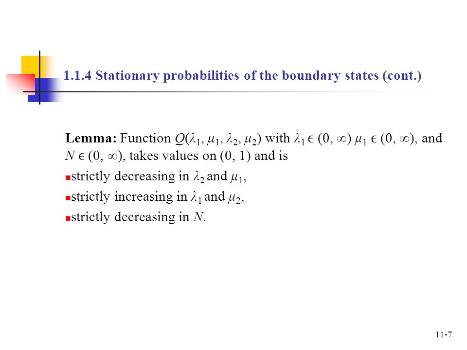
7. 1.1.4 Stationary probabilities of the boundary states (cont.) Lemma: Function Q(λ 1, μ 1, λ 2, μ 2 ) with λ 1 (0, ∞) μ 1 (0, ∞), and N (0, ∞), takes values on (0, 1) and is strictly decreasing in λ 2 and μ 1, strictly increasing in λ 1 and μ 2, strictly decreasing in N. 11-7

8. 1.1.5 Stationary marginal pdf of buffer occupancy 11-8

9. Illustration: Lines with identical e i ’s: 11-9 1.1.5 Stationary marginal pdf of buffer occupancy (cont.)

10. Reversed lines with identical e i ’s: 11-10

11. 1.1.5 Stationary marginal pdf of buffer occupancy (cont.) Reversed lines with non-identical e i ’s: 11-11

12. 1.1.6 Formulas for performance measures Production rate 11-12

13. 1.1.6 Formulas for performance measures (cont.) 11-13 Work-in-process where

14. 1.1.6 Formulas for performance measures (cont.) 11-14 Blockages and starvations i.e., (Recall that for Bernoulli lines, PR = p 1 – BL 1 = p 2 – ST 2.)

15. 1.1.7 Effects of up- and downtime Theorem: Consider lines l 1 and l 2, with machines of identical efficiency and finite buffers of identical capacity. Assume Then, This phenomenon is due to the fact that finite buffers accommodate shorter downtime easier than longer ones 11-15

16. 1.1.7 Effect of up- and downtime (cont.) Note that for an isolated machine, increasing T up by any factor or decreasing T down by the same factor has the same effect: The situation is different for serial lines: Theorem: In synchronous exponential two-machine lines defined by assumptions (a)-(e), PR has a larger increase when the downtime of a machine is decreased by a factor (1 + α), α > 0, than when the uptime is increased by the same factor. 11-16

17. 1.1.8 Asymptotic properties Theorem: 11-17

18. 1.1.8 Asymptotic properties (cont.) Illustration (for the six lines used in the illustration of pdf’s) 11-18

19. 1.2 M > 2-machine case 1.2.1 Mathematical description and aggregation preliminaries Conventions: The same as in two-machine case. States: Too complex – aggregation is used for simplification. 11-19

20. 1.2.1 Mathematical description and aggregation preliminaries (cont.) Backward aggregation 11-20

21. 1.2.1 Mathematical description and aggregation preliminaries (cont.) Forward aggregation 11-21

22. 1.2.2 Aggregation equations with initial conditions: and boundary conditions: 11-22

23. 1.2.2 Aggregation equations (cont.) 11-23 Convergence Theorem: All four sequences are convergent: Moreover, i.e.,

24. 1.2.2 Aggregation equations (cont.) 11-24 Interpretation of the limits: i = 2,…, M – 1

25. 1.2.3 Formulas for performance measures Production rate: Work-in-process 11-25

26. 1.2.3 Formulas for performance measures (cont.) Blockages and starvations: 11-26

27. 1.2.4 PSE Toolbox 11-27

28. 1.2.5 Effects of up- and downtime Remain the same as in two-machine exponential lines: Shorter up- and downtime lead to larger than longer ones, even if the machine efficiencies remain the same. Decreasing T down by any factor leads to a larger than increasing T up by the same factor. 11-28

29. 1.2.6 Asymptotic properties 11-29

30. 1.2.6 Asymptotic properties (cont.) Illustration (Line 1) 11-30

31. 1.2.7 Accuracy of estimates is typically evaluated with the error within 1%. and have lower accuracy. 11-31

32. 1.2.8 System-theoretic properties Theorem: Synchronous exponential lines are reversible: Theorem: is strictly monotonically increasing in μ i, i = 1,…, M, and N i, i = 1,…, M – 1; strictly monotonically decreasing in λ i, i = 1,…, M. 11-32

33. 2. Asynchronous Exponential Lines 2.1 Two-machine case 11-33 c i [parts/min], λ i [1/min], μ i [1/min] TP [parts/min]

34. 2.1.1 Mathematical description Conventions (a)-(e) are assumed to hold. States are the same as in synchronous lines. Analysis is based on continuous time, mixed space Markov processes. Calculations are a little more involved than in the synchronous case. Function Q does not emerge in these calculations. 11-34

35. 2.1.2 Stationary marginal pdf of buffer occupancy 11-35 where

36. 2.1.2 Stationary marginal pdf of buffer occupancy (cont.) 11-36

37. 2.1.2 Stationary marginal pdf of buffer occupancy (cont.) 11-37

38. 2.1.2 Stationary marginal pdf of buffer occupancy (cont.) Illustration 11-38

39. 2.1.2 Stationary marginal pdf of buffer occupancy (cont.) 11-39

40. 2.1.2 Stationary marginal pdf of buffer occupancy (cont.) Observations remain the same as in the synchronous case: Reversibility holds. Larger up- and downtime qualitatively change pdf’s as compared with shorter ones. 11-40

41. 2.1.3 Formulas for performance measures 11-41 Throughput:

42. 2.1.3 Formulas for performance measures (cont.) Work-in-process 11-42

43. 2.1.3 Formulas for performance measures (cont.) Blockages and starvations Represent Denote Then 11-43

44. 2.1.3 Formulas for performance measures (cont.) Using conditional probability formula 11-44

45. 2.1.3 Formulas for performance measures (cont.) Similar arguments are used to calculate BL 1. 11-45

46. 2.1.4 Effects of up- and downtime 11-46 Similar to those in the synchronous case: Larger up- and downtime lead to lower TP than shorter ones. It is more efficient to decrease T down than to increase T up.

47. 2.1.5 Asymptotic properties 11-47

48. 2.1.5 Asymptotic properties (cont.) 11-48

49. 2.1.5 Asymptotic properties (cont.) Observations remain the same as in the synchronous case: WIP may grow almost linearly in N, while TP is always saturating; thus, large N's are not advisable (see Chapter 14). Reverse lines have identical TP. Longer up- and downtime result in lower TP than shorter up- and downtime; in some cases, the difference is as large as 25%. 11-49

50. 2.2 M > 2-machine case Approach: Aggregation procedure based on c i, bl i, and st i. 11-50

51. 2.2.1 Aggregation equations 11-51 with initial conditions and boundary conditions

52. 2.2.1 Aggregation equations (cont.) 11-52 Convergence Theorem: The aggregation procedure is convergent: In addition,

53. 2.2.1 Aggregation equations (cont.) 11-53 Interpretation of and i = 2,…, M – 1

54. 2.2.2 Formulas for performance measures 11-54 Throughput or use the formulas for two-machine lines with and. Work-in-process For, use the two-machine formulas with and. Blockages and starvations

55. 2.2.3 PSE Toolbox 11-55

56. 2.2.4 Effects of up- and downtime Remain the same as in synchronous lines. 11-56

57. 2.2.5 Asymptotic properties → min{c i e i } → 0 → c M e M – 11-57

58. 2.2.5 Asymptotic properties (cont.) Illustration 11-58

59. 2.2.5 Asymptotic properties (cont.) 11-59

60. 2.2.6 Accuracy of the estimates Lower than that for synchronous lines. ε TP is on the average within 5%. ε WIP is on the average within 8%. ε ST i and ε BL i is on the average within 0.03. 11-60

61. 3. Case Studies 3.1 Automotive ignition coil processing system To account for the closed nature of the line, e 1 and T down, 1 have been modified to 0.9226 and 19.12, respectively. 11-61

62. 3.1.1 Model validation 11-62

63. 3.1.2 Effect of starvation by pallets Observation: No significant TP improvement if the closed line is unimpeding. 11-63

64. 3.1.3 Effect of increased buffer capacity and m 9-10 efficiency Observation: Substantial improvement (similar to that obtained using the Bernoulli description) 11-64

65. 3.2 Crankshaft production line (evaluation of the initial description) 11-65 3.2.1 Layout

66. 3.2.2 Structural model 11-66

67. 3.2.3 Machine and buffer parameters 11-67

68. 3.2.4 Performance and “what if” analysis Sensitivity to buffer capacity Sensitivity to Sta. 7 efficiency Observation: Although the initial design meets specification, Sta. 7’s performance should be given a particular attention in order to maintain the production goal. 11-68

69. 4. Summary The performance measures of serial lines with exponential machines can be evaluated using the same approach as in the Bernoulli case. Specifically, two-machines lines can be evaluated by closed-form expressions, and aggregation procedures can be used to analyze longer lines. However, all analytical expressions are more involved, especially in the asynchronous case. Stationary marginal pdf's of buffer occupancy contain δ- functions, which account for buffers being empty and full. The accuracy of the resulting performance measure estimates in the synchronous case is similar to that of the Bernoulli case. In the asynchronous case, the accuracy is lower. 11-69

70. Shorter up- and downtime lead to a higher production rate (or throughput) than longer ones, even if machine efficiency remains constant. A decrease of the downtime leads to higher throughput of a serial line than an equivalent increase of the uptime. Exponential lines observe the usual monotonicity and reversibility properties. 11-70 4. Summary (cont.)