1. Design & Analysis of Algorithms CS315
Decrease & Conquer
Design & Analysis of Algorithms CS315

2. Decrease-and-Conquer
Reduce problem instance to smaller instance of the same problem
Solve smaller instance
Extend solution of smaller instance to obtain solution to original instance
Can be implemented either top-down or bottom-up
Also referred to as inductive or incremental approach

3. 3 Types of Decrease and Conquer
Decrease by a constant (usually by 1)
Decrease by a constant factor (usually by half)
Variable-size decrease

4. Decrease by a constant :
Insertion sort
Topological sorting
Algorithms for generating permutations, subsets

5. Decrease by a constant factor
Binary search and bisection method
Exponentiation by squaring
Multiplication à la russe

6. Variable-size decrease
Euclid’s algorithm
Selection by partition
Nim-like games

7. Problem: Compute an
Try to get the students involved in coming up with these:
Brute Force:
an= a*a*a*a*...*a n
Divide and conquer:
an= an/2 * an/2 (more accurately, an= an/2 * a n/2│)
Decrease by one:
an= an-1* a (one hopes a student will ask what is the difference with brute force here:
there is none in the resulting algorithm, of course, but you can arrive
at it in two different ways)
Decrease by constant factor:
an= (an/2) (again, if no student asks about it, be sure to point out the difference
with divide and conquer. Here there is a significant difference that leads to a
much more efficient algorithm – in divide and conquer we recompute an/2

8. Problem: Compute an
Try to get the students involved in coming up with these:
Brute Force:
an= a*a*a*a*...*a n
Divide and conquer:
an= an/2 * an/2 (more accurately, an= an/2 * a n/2│)
Decrease by one:
an= an-1* a (one hopes a student will ask what is the difference with brute force here:
there is none in the resulting algorithm, of course, but you can arrive
at it in two different ways)
Decrease by constant factor:
an= (an/2) (again, if no student asks about it, be sure to point out the difference
with divide and conquer. Here there is a significant difference that leads to a
much more efficient algorithm – in divide and conquer we recompute an/2

9. Insertion Sort
To sort array A[0..n-1], sort A[0..n-2] recursively and then insert A[n-1] in its proper place among the sorted A[0..n-2]
Usually implemented bottom up (non-recursively)

10. Pseudocode of Insertion Sort

11. Insertion Sort Example:
Elements are percolated down to their appropriate position 6 4 1 8 5 4 6 1 8 5 1 4 6 8 5 1 4 6 8 5 1 4 5 6 8

12. Analysis of Insertion Sort
Space efficiency: in-place
Stability: yes
Best elementary sorting algorithm overall
Binary insertion sort

13. Analysis of Insertion Sort
Time efficiency: Worst case
Cworst(n) = n(n-1)/2  Θ(n2)
Each element must be compared to all preceding elements

14. Analysis of Insertion Sort
Time efficiency: Best case Cbest(n) = n - 1  Θ(n) (also fast on almost sorted arrays)
Only one comparison is necessary for each element

15. Analysis of Insertion Sort
Time efficiency: Average case Cavg(n) ≈ n2/4  Θ(n2)
Given that that there is an equal likelihood that an element will be compared to 1, 2, … , (i-1) elements, the average case is the average of the best and worst case
Note: The above is NOT true for all algorithms

16. Dags and Topological Sorting
A dag: a directed acyclic graph, i.e. a directed graph with no (directed) cycles
Arise in modeling many problems that involve prerequisite
constraints (construction projects, document version control)
Vertices of a dag can be linearly ordered so that for every edge its starting vertex is listed before its ending vertex (topological sorting). Being a dag is also a necessary condition for topological sorting be possible. a b a b
Not a DAG
DAG c d c d

17. Topological Sorting Example
Order the following items in a food chain
tiger
human
fish
sheep
shrimp
plankton
wheat

18. DFS-based Algorithm DFS-based algorithm for topological sorting
Perform DFS traversal, noting the order vertices are popped off the traversal stack
Reverse order solves topological sorting problem
Back edges encountered?→ NOT a dag!
Example: a b c d e f g h

19. Source Removal Algorithm
Repeatedly identify and remove a source (a vertex with no incoming edges) and all the edges incident to it until either no vertex is left (problem is solved) or there is no source among remaining vertices (not a dag)
Example:
Efficiency: same as efficiency of the DFS-based algorithm a b c d e f g h

20. Generating Permutations
Minimal-change decrease-by-one algorithm
If n = 1 return 1; otherwise, generate recursively the list of all permutations of 12…n-1 and then insert n into each of those permutations by starting with inserting n into 12...n-1 by moving right to left and then switching direction for each new permutation
Example: n=3
start 1
insert 2 into 1 right to left 12 21
insert 3 into 12 right to left
insert 3 into 21 left to right

21. Other permutation generating algorithms
Johnson-Trotter (p. 145)
Lexicographic-order algorithm (p. 146)
Heap’s algorithm (Problem 4 in Exercises 4.3)

22. Generating Subsets
Binary reflected Gray code: minimal-change algorithm for generating 2n bit strings corresponding to all the subsets of an n-element set where n > 0
If n=1 make list L of two bit strings 0 and 1
else
generate recursively list L1 of bit strings of length n-1
copy list L1 in reverse order to get list L2
add 0 in front of each bit string in list L1
add 1 in front of each bit string in list L2
append L2 to L1 to get L
return L

23. Decrease-by-Constant-Factor Algorithms
In this variation of decrease-and-conquer, instance size is reduced by the same factor (typically, 2)
Examples:
binary search and the method of bisection
exponentiation by squaring
multiplication à la russe (Russian peasant method)
fake-coin puzzle
Josephus problem

24. Binary Search Very efficient algorithm for searching in sorted array:K
versus
A[0] A[m] A[n-1]
If K = A[m], stop (successful search); otherwise, continue
searching by the same method in A[0..m-1] if K < A[m]
and in A[m+1..n-1] if K > A[m]
l  0; r  n-1
while l  r do
m  (l+r)/2
if K = A[m] return m
else if K < A[m] r  m-1
else l  m+1
return -1

25. Analysis of Binary Search
Time efficiency
worst-case recurrence: Cw (n) = 1 + Cw( n/2 ), Cw (1) = 1 solution: Cw(n) = log2(n+1) This is VERY fast: e.g., Cw(106) = 20
Optimal for searching a sorted array
Limitations: must be a sorted array (not linked list)
Bad (degenerate) example of divide-and-conquer
Has a continuous counterpart called bisection method for solving equations in one unknown f(x) = 0 (see Sec. 12.4)

26. Exponentiation by Squaring
The problem: Compute an where n is a nonnegative integer The problem can be solved by applying recursively the formulas:
For even values of n
a n = (a n/2 )2 if n > 0 and a 0 = 1
For odd values of n
a n = (a (n-1)/2 )2 a
Recurrence: M(n) = M( n/2 ) + f(n), where f(n) = 1 or 2,
M(0) = 0
Master Theorem: M(n)  Θ(log n) = Θ(b) where b = log2(n+1)

27. Russian Peasant Multiplication
The problem: Compute the product of two positive integers Can be solved by a decrease-by-half algorithm based on the following formulas.
For even values of n:
n 2
n * m = * 2m
For odd values of n:
n – 1 2
n * m = * 2m + m if n > 1 and m if n = 1

28. Russian Peasant Multiplication
Compute 20 * 26 n m
520
Note: Method reduces to adding m’s values corresponding to odd n’s.

29. Fake-Coin Puzzle (simpler version)
Given:
There are n identically looking coins one of which is fake.
There is a balance scale but there are no weights; the scale can tell whether two sets of coins weigh the same and, if not, which of the two sets is heavier (but not by how much).
Design an efficient algorithm for detecting the fake coin. Assume that the fake coin is known to be lighter than the genuine ones.

30. Variable-Size-Decrease Algorithms
In the variable-size-decrease variation of decrease-and-conquer, instance size reduction varies from one iteration to another
Examples:
Euclid’s algorithm for greatest common divisor
partition-based algorithm for selection problem
interpolation search
some algorithms on binary search trees
Nim and Nim-like games

31. Euclid’s Algorithm
Euclid’s algorithm is based on repeated application of equality gcd(m, n) = gcd(n, m mod n)
Example: gcd(80,44) = gcd(44,36) = gcd(36, 12) = gcd(12,0) = 12
One can prove that the size, measured by the second number, decreases at least by half after two consecutive iterations.
Hence, T(n)  O(log n)

32. Selection Problem
Find the k-th smallest element in a list of n numbers
k = 1 or k = n
median: k = n/2
Example: 4, 1, 10, 9, 7, 12, 8, 2, median = ?
The median is used in statistics as a measure of an average
value of a sample. In fact, it is a better (more robust) indicator
than the mean, which is used for the same purpose.

33. Digression: Post Office Location Problem
Given n village locations along a straight highway, where should a new post office be located to minimize the average distance from the villages to the post office?

34. Algorithms for the Selection Problem
The sorting-based algorithm: Sort and return the k-th element Efficiency (if sorted by mergesort): Θ(nlog n)
A faster algorithm is based on the array partitioning:
Assuming that the array is indexed from 0 to n-1 and s is a split position obtained by the array partitioning:
If s = k-1, the problem is solved;
if s > k-1, look for the k-th smallest element in the left part; if s < k-1, look for the (k-s)-th smallest element in the right part.
Note: The algorithm can simply continue until s = k-1. s
all are ≤ A[s]
all are ≥ A[s]

35. Two Partitioning Algorithms
There are two principal ways to partition an array:
One-directional scan (Lomuto’s partitioning algorithm)
Two-directional scan (Hoare’s partitioning algorithm)

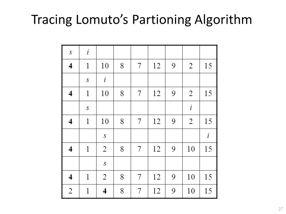
36. Lomuto’s Partitioning Algorithm
Scans the array left to right maintaining the array’s partition into three contiguous sections: < p,  p, and unknown, where p is the value of the first element (the partition’s pivot).
On each iteration the unknown section is decreased by one element until it’s empty and a partition is achieved by exchanging the pivot with the element in the split position s.

37. Tracing Lomuto’s Partioning Algorithm4 1 10 8 7 12 9 2 15

38. Tracing Quickselect (Partition-based Algorithm)
Find the median of 4, 1, 10, 9, 7, 12, 8, 2, 15
Here: n = 9, k = 9/2 = 5, k -1=4
After 1st partitioning: s=2<k-1=4 1 2 3 4 5 6 7 8 10 12 9 15
After 2nd partitioning: s=4=k-1
The median is A[4]= 8

39. Efficiency of Quickselect
Average case (average split in the middle):
C(n) = C(n/2)+(n+1) C(n)  Θ(n)
Worst case (degenerate split): C(n)  Θ(n2)
A more sophisticated choice of the pivot leads to a complicated algorithm with Θ(n) worst-case efficiency.

40. x = l + (v - A[l])(r - l)/(A[r] – A[l] )
Interpolation Search
Searches a sorted array similar to binary search but estimates location of the search key in A[l..r] by using its value v. Specifically, the values of the array’s elements are assumed to grow linearly from A[l] to A[r] and the location of v is estimated as the x-coordinate of the point on the straight line through (l, A[l]) and (r, A[r]) whose y-coordinate is v:
x = l + (v - A[l])(r - l)/(A[r] – A[l] )

41. Analysis of Interpolation Search
Efficiency
average case: C(n) < log2 log2 n + 1
worst case: C(n) = n
Preferable to binary search only for VERY large arrays and/or expensive comparisons
Has a counterpart, the method of false position (regula falsi), for solving equations in one unknown (Sec. 12.4)

42. Binary Search Tree Algorithms
Several algorithms on BST requires recursive processing of just one of its subtrees, e.g.,
Searching
Insertion of a new key
Finding the smallest (or the largest) key k
<k
>k

43. Searching in Binary Search Tree
Algorithm BTS(x, v) //Searches for node with key equal to v in BST rooted at node x if x = NIL return -1 else if v = K(x) return x else if v < K(x) return BTS(left(x), v) else return BTS(right(x), v) Efficiency worst case: C(n) = n average case: C(n) ≈ 2ln n ≈ 1.39log2 n

44. One-Pile Nim
Rules:
There is a pile of n chips
Two players take turn by removing from the pile at least 1 and at most m chips. (The number of chips taken can vary from move to move.)
The winner is the player that takes the last chip
Who wins the game? The player moving first or second, assuming both players make the best moves possible?
It’s a good idea to analyze this and similar games “backwards”, i.e., starting with n = 0, 1, 2, …

45. Partial Graph of One-Pile Nim with m = 4
Vertex numbers indicate n, the number of chips in the pile. The losing position for the player to move are circled. Only winning moves from a winning position are shown (in bold).
Generalization: The player moving first wins iff n is not a multiple of 5 (more generally, m+1); the winning move is to take n mod 5 (n mod (m+1)) chips on every move.