Download presentation
Presentation is loading. Please wait.

1
Cuong Cao Pham and Jae Wook Jeon, Member, IEEE
Domain Transformation-Based Efficient Cost Aggregation for Local Stereo Matching Cuong Cao Pham and Jae Wook Jeon, Member, IEEE IEEE Transactions on Circuits and Systems for Video Technology, 2012

2
Outline Introduction Framework Proposed Algorithm Experimental Results
Compute Costs Cost Aggregation : Domain Tramsformation Optimization & Refinment Experimental Results Conclusion

3
Introduction

4
Background Global stereo algorithms: Local stereo algorithms :
[4] K.-J. Yoon and I.-S. Kweon, “Adaptive Support-Weight Approach for Correspondence Search,” IEEE Trans. Pattern Anal. Mach. Intell., vol.28, no. 4, pp , 2006. Global stereo algorithms: High accuracy but low speed Local stereo algorithms : High speed but low accuracy The key : cost aggregation Adaptive support-weight[4] : ‧The most well-known local method ‧The state-of-art local algorithm ‧Reduce the gap between global method and local method → Excessive time consumption related to support window size

5
Related Work Adaptive Weight[4] Cost-volume filtering[21]
Bilateral filter Cost-volume filtering[21] Guided filter Geodesic Diffusion[27] Anisotropic diffusion → Geodesic diffusion [21] C. Rhemann, A. Hosni, M. Bleyer, C. Rother, and M. Gelautz, “Fast Cost-Volume Filtering for Visual Correspondence and Beyond,” in Proc.IEEE Intl. Conf. Comput. Vis. Pattern Recognit. (CVPR), pp ,2011. [27] L. De-Maeztu, A. Villanueva, and R. Cabeza, “Near Real-Time Stereo Matching Using Geodesic Diffusion,” IEEE Trans. Pattern Anal. Mach. Intell., vol. 34, no. 2, pp , 2012.
![Related Work Adaptive Weight[4] Cost-volume filtering[21]](http://slideplayer.com/slide/4443022/14/images/5/Related+Work+Adaptive+Weight%5B4%5D+Cost-volume+filtering%5B21%5D.jpg "Bilateral filter. Cost-volume filtering[21] Guided filter. Geodesic Diffusion[27] Anisotropic diffusion. → Geodesic diffusion. [21] C. Rhemann, A. Hosni, M. Bleyer, C. Rother, and M. Gelautz, Fast Cost-Volume Filtering for Visual Correspondence and Beyond, in Proc.IEEE Intl. Conf. Comput. Vis. Pattern Recognit. (CVPR), pp ,2011. [27] L. De-Maeztu, A. Villanueva, and R. Cabeza, Near Real-Time Stereo Matching Using Geodesic Diffusion, IEEE Trans. Pattern Anal. Mach. Intell., vol. 34, no. 2, pp ,")
6
Objective Present a cost aggregation technique: Domain transformation:
Achieve high precision Fast execution Using Domain transformation Domain transformation: Aggregation of 2D cost data → a sequence of 1D filters Lower computational requirements

7
Framework

8
Framework

9
Proposed Algorithm

10
Pixel-wise Cost Consumption
Truncated absolute difference (TAD) : TAD of the gradient : Final cost data: Ii(p): intensity value of the i-th color channel in the RGB color space at pixel p of the image I Tc : user-defined truncation value
![]()
11
Aggregation 1D Cost Data
Inspired by the domain transformation technique[14] Dimensionality reduction technique Defines a geodesic distance-preserving representation of a 2D image embedded in 5D (x, y, Ir, Ig, Ib) as a real line. Aggregation of 2D cost data → a sequence of 1D filters Reduce computational time [14] Eduardo S. L. Gastal and Manuel M. Oliveira, “Domain Transform for Edge-Aware Image and Video Processing,” ACM Trans. Graph., vol. 30, no. 4, 2011.
 as a real line. Aggregation of 2D cost data → a sequence of 1D filters. Reduce computational time. [14] Eduardo S. L. Gastal and Manuel M. Oliveira, Domain Transform for Edge-Aware Image and Video Processing, ACM Trans. Graph., vol. 30, no. 4,")
12
Aggregation 1D Cost Data
1D discrete signal: Cost slide Cd : Feedback comb filter[32]: Cd,y : input signal Cd,y : output signal a ∈ 0,1 : feedback coefficient row y a : consistent → non-edge-aware filter ‘ n-1 n [32] J. Smith, “Introduction to Digital Filters with Audio Applications,” W3K Publishing, 2007.

13
Aggregation 1D Cost Data
1D discrete signal: Cost slide Cd : Feedback comb filter[32]: Cd,y : input signal Cd,y : output signal a ∈ 0,1 : feedback coefficient row y a : consistent → non-edge-aware filter ‘ n-1 n

14
Aggregation 1D Cost Data
Two similar samples set a high value of a Two different samples set a low value of a ( Discontinue region → prevent the propagation train ) Edge-aware feedback comb filter: g : chosen metric representing the dissimilarity between two samples Compute g as the distance between two samples in the 1D domain (transformed from the corresponding row of the guidance image I)
 Edge-aware feedback comb filter: g : chosen metric representing the dissimilarity between two samples. Compute g as the distance between two samples in the 1D domain. (transformed from the corresponding row of the guidance image I)")
15
Domain Transformation
I : Ω ϲ R2 → R3 (a 2D RGB color image) p = (xp, yp) : spatial coordinate I(p) = (rp, gp, bp) : range coordinates Goal: find a transform t :R2 → R which preserves the original distances between points on C (given by some metric) R2 R3 g v
 p = (xp, yp) : spatial coordinate. I(p) = (rp, gp, bp) : range coordinates. Goal: find a transform t :R2 → R which preserves the original distances between points on C (given by some metric) R2. R3. g. v.")
16
Domain transformation
L1 distance between two neighboring points in the original domain R2 Distance between two corresponding samples in the new domain R gt(x) = t (x, I(x)) : the transformation operator at point x must equal R R2
 = t (x, I(x)) : the transformation operator at point x. must equal. R. R2.")
17
Domain transformation
Divide both sides by h and take the limit as h→0: The value at any point u in the transformed domain: (By taking the integral of gt′ (x) from 0 to u)
 from 0 to u)")
18
Domain transformation
The value at any point u in the transformed domain: The distance between any two points u and v in the transformed domain : (corresponds to the arc length from u to v of the signal I)
")
19
Domain transformation
The distance between any two points u and v : We can also control the influence of spatial and intensity range information similar to the bilateral filter. Embedding the values of σs and σr :

20
Domain transformation
Select the maximum absolute difference to define the distance between two points in the original domain: The final distance g:

21
Domain transformation
Left image Non-edge-aware filter Edge-aware filter

22
Aggregation 2D Cost Data

23
Aggregation 2D Cost Data
1. Left → Right 2. Right → Left 3. Top → Bottom 4. Bottom→ Top

24
Aggregation 2D Cost Data
L→ R R→ L T→ B B→ T

25
Aggregation 2D Cost Data
is the 1D discrete signal plotted from each column along the y direction of the cost slide Cd : σH : kernel standard deviation (implicitly set to σs) σs ∈ [10,300] and σr ∈ [0.01,0.3] can yields good results.
 σs ∈ [10,300] and σr ∈ [0.01,0.3] can yields good results.")
26
Aggregation 2D Cost Data
‧Algorithm:

27
Optimization & Refinement
Winner-take-all Select disparities Left-Right consistency check Occluded regions Weighted median filter Noise removing

28
Winner-take-all Winner-take-all(WTA) strategy:
Sd : the set of all possible disparities Cd : Aggregated cost ‘

29
Left-right consistency check
The disparity maps obtained at this stage contain errors in the occluded regions. Perform Left-right consistency check A pixel in the left disparity map is marked as invalidated: when its value differs from the corresponding value of the pixel in the right disparity map by a value greater than one Assign the minimum value between two closest validated pixels min validated Left image Right image invalidated

30
Weighted Median Filter
Using a weighted median filter to : Remove streak-like artifacts Remove the small amount of remaining noise Select bilateral filter weight to compute the weighted median filter The validated pixels are not affected by this operation.

31
Consistency Map vs. Final disparity
Invalidated pixels

32
Experimental Results

33
Experimental Results Middlebury stereo evaluation Real-world image
Middlebury dataset Real-world image Camcorder data Execution time CUDA implementation

34
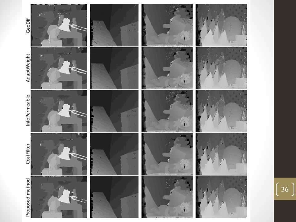
Middlebury Evaluation - 1
Adaptive Weight[4] 35×35 support window with γs = 17 and γr = 7:5 Cost-volume filtering[21] 19×19 support window and ε = 0:0004 Geodesic Diffusion[27] Iterated n = 24 times with γc = 40 and l0 = 0:15 InfoPermeable[31] Exponential function with σ = 25 Proposed σs=25 and σr=0.1 Compare with the best-performing algorithm inspired by well-known edge-aware filters [31] C. Cigla and A. A. Alatan, “Efficient Edge-Preserving Stereo Matching”, in ICCV Workshop on LDRMV, 2011.

35
Middlebury Evaluation - 1
Compare the performance of the raw cost aggregation The same pixel-wise cost computation and disparity optimization steps were installed to ensure fair comparison. Select the TAD of the color and the gradient for computing matching costs { λ , Tc, Tg }={ 0.1, 7/255, 2/255 } Guidance image used for the aggregation stage: Using 3x3 median filter Reduce the high-frequncy information that is not actually useful

37
Experimental Results Only non-occluded and discontinuity regions

38
Middlebury Evaluation - 2
Without refinement vs. with refinement { λ , Tc, Tg, σs , σr }={ 0.1, 7/255, 2/255, 45, } 3x3 median filter Filtering Guidance image used for the aggregation stage The weighted median filter Used in disparity refinement stage r = 21, γs = 81, and γr = 0.04

39
Experimental Results without refinement with refinement

40
Experimental Results

41
Experimental Results

42
Experimental Results

43
Real-world Image Camcorder data:
Cafe (640×360, 32 possible disparities) Newspaper (512×384, 32 possible disparities) Book_Arrival (512×384, 60 possible disparities)
 Newspaper (512×384, 32 possible disparities) Book_Arrival (512×384, 60 possible disparities)")
44
Proposed vs. CostFilter[21]
![Proposed vs. CostFilter[21]](http://slideplayer.com/slide/4443022/14/images/44/Proposed+vs.+CostFilter%5B21%5D.jpg "Proposed vs. CostFilter[21]")
45
Execution time Using C++
PC with an AMD Athlon 64 X2 Dual Core Ghz. Measure only the execution time of the aggregation performing on the left view No occlusion handling or post-processing times were included.

46
Execution time Iteration times: n Window: 2n+1 × 2n+1
Support window size / number of iterations

47
CUDA Implementation Algorithm Time(s) Graphics Card Image GeoDif 0.06
NVIDIA GeForce GTX 480 Tsukuba stereo pair CostFilter 0.041 400×300 image Proposed 0.0095 NVIDIA GeForce GTX 460 Tsukuba stereo pair

48
Conclusion

49
Conclusion Solve the excessive time consumption bottleneck of adaptive-weight Integrates the appealing properties of domain transformation into the cost aggregation Using a sequence of 1D operations Lower computational requirements Lower memory costs Fast and accurate local method

Similar presentations


, I. Grinias (2) and G. Tziritas (3) 07-07-2009.>")


 Shengcai Liao, Guoying Zhao, Vili Kellokumpu,>")
 22–32.>")


![100+ Times Faster Weighted Median Filter [cvpr ‘14]](/17/5282204/big_thumb.jpg "100+ Times Faster Weighted Median Filter [cvpr ‘14]>")


