1. Motion Estimation I What affects the induced image motion? Camera motion Object motion Scene structure

2. Example Flow Fields This lesson – estimation of general flow-fields Next lesson – constrained by global parametric transformations

3. The Aperture Problem So how much information is there locally…?

4. The Aperture Problem Copyright, 1996 © Dale Carnegie & Associates, Inc. Not enough info in local regions

5. The Aperture Problem Copyright, 1996 © Dale Carnegie & Associates, Inc. Not enough info in local regions

6. The Aperture Problem Copyright, 1996 © Dale Carnegie & Associates, Inc.

7. The Aperture Problem Copyright, 1996 © Dale Carnegie & Associates, Inc. Information is propagated from regions with high certainty (e.g., corners) to regions with low certainty.

8. Such info propagation can cause optical illusions… Illusory corners

9. 1. Gradient-based (differential) methods (Horn &Schunk, Lucase & Kanade) 2. Region-based methods (Correlation, SSD, Normalized correlation) Direct (intensity-based) Methods Feature-based Methods

10. Image J (taken at time t) Brightness Constancy Assumption Image I (taken at time t+1)

11. Brightness Constancy Equation: The Brightness Constancy Constraint Linearizing (assuming small (u,v)):

12. Observations: Need additional constraints…

13. Horn and Schunk (1981) Add global smoothness term Smoothness error Error in brightness constancy equation Minimize: Solve by using calculus of variations

14. Horn and Schunk (1981) Inherent problems: * Smoothness assumption wrong at motion/depth discontinuities  over-smoothing of the flow field. * How is Lambda determined…?

15. Lucas-Kanade (1984) Assume a single displacement (u,v) for all pixels within a small window (e.g., 5x5) Minimize E(u,v): Geometrically -- Intersection of multiple line constraints Algebraically --

16. Lucas-Kanade (1984) Differentiating w.r.t u and v and equating to 0: Solve for (u,v) [ Repeat this process for each and every pixel in the image ] Minimize E(u,v):

17. Singularites Where in the image will this matrix be invertible and where not…?  Homework

18. Linearization approximation  iterate & warp x x0x0 Initial guess: Estimate: estimate update

19. x x0x0 Initial guess: Estimate: Linearization approximation  iterate & warp

20. x x0x0 Initial guess: Estimate: Initial guess: Estimate: estimate update Linearization approximation  iterate & warp

21. x x0x0

22. Revisiting the small motion assumption Is this motion small enough? Probably not—it’s much larger than one pixel (2 nd order terms dominate) How might we solve this problem?

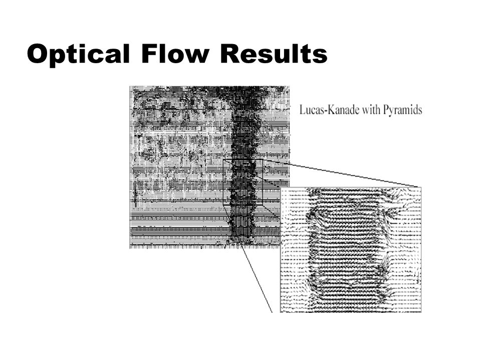
23. ==> small u and v... u=10 pixels u=5 pixels u=2.5 pixels u=1.25 pixels image I image J iterate refine + Pyramid of image JPyramid of image I image I image J Coarse-to-Fine Estimation Advantages: (i) Larger displacements. (ii) Speedup. (iii) Information from multiple window sizes.

24. Optical Flow Results

26. Inherent problems: * Still smoothes motion discontinuities (but unlike Horn & Schunk, does not propagate error across the entire image) * Local singularities (due to the aperture problem) Lucas-Kanade (1984) Maybe increase the aperture (window) size…? But no longer a single motion…  Global parametric motion estimation – next week.

27. 1. Gradient based methods (Horn &Schunk, Lucase & Kanade, …) 2. Region based methods (SSD, Normalized correlation, etc.) Copyright, 1996 © Dale Carnegie & Associates, Inc. But… (despite coarse-to-fine estimation) rely on B.C. cannot handle very large motions (no more than 10%-15% of image width/height) small object moving fast…?

28. Region-Based Methods * Define a small area around a pixel as the region. * Match the region against each pixel within a search area in next image. * Use a match measure (e.g., SSD=sum of-squares difference, NC=normalized correlation, etc.) * Choose the maximum (or minimum) as the match. Advantages: Can avoid B.C. assumption Can handle large motions (even of small objects) Disadvantages: Less accurate (smaller sub-pixel accuracy) Computationally more expensive

29. Wu, Rubinstein, Shih, Guttag, Durand, Freeman “Eulerian Video Magnification for Revealing Subtle Changes in the World”, SIGGRAPH 2012 Motion Magnification Result: baby-iir-r1-0.4-r2-0.05-alpha-10-lambda_c-16-chromAtn-0.1.mp4 baby-iir-r1-0.4-r2-0.05-alpha-10-lambda_c-16-chromAtn-0.1.mp4 Source video: baby.mp4 baby.mp4 Paper + videos can be found on: http://people.csail.mit.edu/mrub/vidmag

30. Motion Magnification Could compute optical flow and magnify it But… very complicated (motions are almost invisible) Alternatively: But holds only for small u s and v s  apply coarse to fine to generate larger motions

31. Motion Magnification What is equivalent to?  This is equivalent to keeping the same temporal frequencies, but magnifying the amplitude (increase frequency coefficient).  Can decide to do this selectively to specific temporal frequencies (e.g., a range of frequencies of expected heart rates).

32. Wu, Rubinstein, Shih, Guttag, Durand, Freeman “Eulerian Video Magnification for Revealing Subtle Changes in the World”, SIGGRAPH 2012 Motion Magnification Paper + videos can be found on: http://people.csail.mit.edu/mrub/vidmag A simplified version of this work  the next programming exercise Exercise will be posted within a few days Meanwhile, please read SIGGRAPH’2012 paper