1. LARGE-SCALE IMAGE PARSING Joseph Tighe and Svetlana Lazebnik University of North Carolina at Chapel Hill road building car sky

2. Small-scale image parsing Tens of classes, hundreds of images He et al. (2004), Hoiem et al. (2005), Shotton et al. (2006, 2008, 2009), Verbeek and Triggs (2007), Rabinovich et al. (2007), Galleguillos et al. (2008), Gould et al. (2009), etc. Figure from Shotton et al. (2009)

3. Large-scale image parsing Hundreds of classes, tens of thousands of images Non-uniform class frequencies

4. Large-scale image parsing Hundreds of classes, tens of thousands of images Evolving training set http://labelme.csail.mit.edu/ Non-uniform class frequencies

5. Challenges  What’s considered important for small-scale image parsing?  Combination of local cues  Multiple segmentations, multiple scales  Context  How much of this is feasible for large-scale, dynamic datasets?

6. Our first attempt: A nonparametric approach  Lazy learning: do (almost) nothing up front  To parse (label) an image we will:  Find a set of similar images  Transfer labels from the similar images by matching pieces of the image (superpixels)

7. Finding Similar Images

8. Ocean Open Field Highway Street Forest Mountain Inner City Tall Building What is depicted in this image? Which image is most similar? Then assign the label from the most similar image

9. Pixels are a bad measure of similarity Most similar according to pixel distanceMost similar according to “Bag of Words”

10. Origin of the Bag of Words model  Orderless document representation:  frequencies of words from a dictionary Salton & McGill (1983) US Presidential Speeches Tag Cloud http://chir.ag/phernalia/preztags/

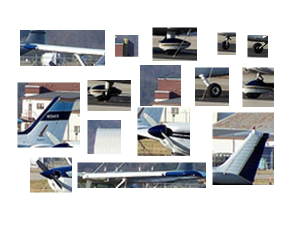
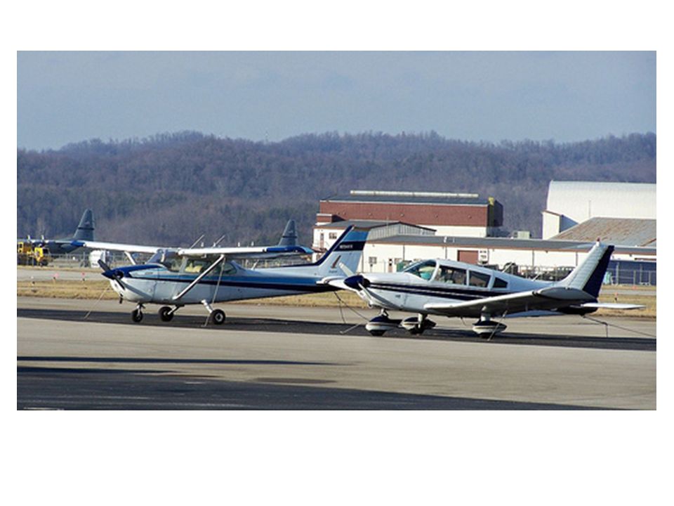
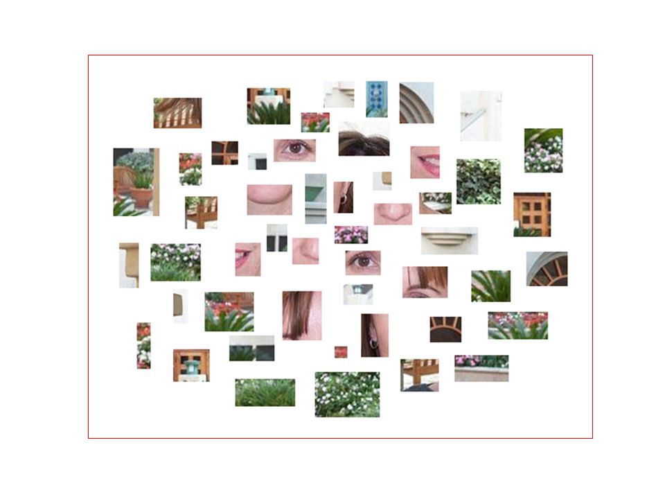
11. What are words for an image?

16. Wing Tail WheelBuildingPropeller

17. Wing Tail WheelBuilding PropellerJet Engine

18. Wing Tail WheelBuilding PropellerJet Engine

19. Wing Tail WheelBuilding PropellerJet Engine

20. But where do the words come from?

23. Then where does the dictionary come from?

24. Example Dictionary Source: B. Leibe

25. Another dictionary … … … … Source: B. Leibe

26. Fei-Fei et al. 2005

27. Outline of the Bag of Words method  Divide the image into patches  Assign a “word” for each patch  Count the number of occurrences of each “word” in the image

28. Does this work for our problem? 65,536 Pixels256 Dimensions

29. Which look the most similar?

30. building road car sky building road car sky building road car sky building road car sky building road car sky tree sky tree building sand mountain car road

31. Step 1: Scene-level matching Gist (Oliva & Torralba, 2001) Spatial Pyramid (Lazebnik et al., 2006) Color Histogram Retrieval set: Source of possible labels Source of region-level matches

32. Step 2: Region-level matching

33. Superpixels (Felzenszwalb & Huttenlocher, 2004)

34. Step 2: Region-level matching Snow Road Tree Building Sky Pixel Area (size)

35. Road Sidewalk Step 2: Region-level matching Absolute mask (location)

36. Step 2: Region-level matching Road SkySnow Sidewalk Texture

37. Step 2: Region-level matching Building Sidewalk Road Color histogram

38. Step 2: Region-level matching Superpixels (Felzenszwalb & Huttenlocher, 2004) Superpixel features

39. Region-level likelihoods  Nonparametric estimate of class-conditional densities for each class c and feature type k:  Per-feature likelihoods combined via Naïve Bayes: kth feature type of ith region Features of class c within some radius of r i Total features of class c in the dataset

40. Region-level likelihoods BuildingCarCrosswalk SkyWindowRoad

41. Step 3: Global image labeling  Compute a global image labeling by optimizing a Markov random field (MRF) energy function: Likelihood score for region r i and label c i Co-occurrence penalty Vector of region labels Regions Neighboring regions Smoothing penalty riri rjrj Efficient approximate minimization using  - expansion (Boykov et al., 2002)

42. Step 3: Global image labeling  How do we resolve issues like this? sky tree sand road sea road Original image Maximum likelihood labeling sky sand sea

43. Step 3: Global image labeling  Compute a global image labeling by optimizing a Markov random field (MRF) energy function: Likelihood score for region r i and label c i Co-occurrence penalty Vector of region labels Regions Neighboring regions Smoothing penalty

44. Step 3: Global image labeling  Compute a global image labeling by optimizing a Markov random field (MRF) energy function: Maximum likelihood labeling Edge penaltiesFinal labelingFinal edge penalties road building car window sky road building car sky Likelihood score for region r i and label c i Co-occurrence penalty Vector of region labels Regions Neighboring regions Smoothing penalty

45. Step 3: Global image labeling  Compute a global image labeling by optimizing a Markov random field (MRF) energy function: sky tree sand road sea road sky sand sea Original image Maximum likelihood labeling Edge penalties MRF labeling Likelihood score for region r i and label c i Co-occurrence penalty Vector of region labels Regions Neighboring regions Smoothing penalty

46. Joint geometric/semantic labeling  Semantic labels: road, grass, building, car, etc.  Geometric labels: sky, vertical, horizontal  Gould et al. (ICCV 2009) sky tree car road sky horizontal vertical Original imageSemantic labelingGeometric labeling

47. Joint geometric/semantic labeling  Objective function for joint labeling: Geometric/semantic consistency penalty Semantic labels Geometric labels Cost of semantic labeling Cost of geometric labeling sky tree car road sky horizontal vertical Original imageSemantic labelingGeometric labeling

48. Example of joint labeling

49. Understanding scenes on many levels To appear at ICCV 2011

50. Understanding scenes on many levels To appear at ICCV 2011

51. Datasets Training imagesTest imagesLabels SIFT Flow (Liu et al., 2009)2,48820033 Barcelona (Russell et al., 2007)14,871279170 LabelMe+SUN50,424300232

52. Datasets Training imagesTest imagesLabels SIFT Flow (Liu et al., 2009)2,48820033 Barcelona (Russell et al., 2007)14,871279170 LabelMe+SUN50,424300232

53. Overall performance SIFT FlowBarcelonaLabelMe + SUN SemanticGeom.SemanticGeom.SemanticGeom. Base73.2 (29.1)89.862.5 (8.0)89.946.8 (10.7)81.5 MRF76.3 (28.8)89.966.6 (7.6)90.250.0 (9.1)81.0 MRF + Joint76.9 (29.4)90.866.9 (7.6)90.750.2 (10.5)82.2 LabelMe + SUN IndoorLabelMe + SUN Outdoor SemanticGeom.SemanticGeom. Base22.4 (9.5)76.153.8 (11.0)83.1 MRF27.5 (6.5)76.456.4 (8.6)82.3 MRF + Joint27.8 (9.0)78.256.6 (10.8)84.1 *SIFT Flow: 74.75

54. Per-class classification rates

55. Results on SIFT Flow dataset

56. 55.392.2 93.6 Results on LM+SUN dataset ImageGround truth Initial semanticFinal semantic Final geometric

57. 58.993.057.3 Results on LM+SUN dataset ImageGround truth Initial semanticFinal semantic Final geometric

58. 11.6 0.0 60.3 93.0 ImageGround truth Initial semanticFinal semantic Final geometric Results on LM+SUN dataset

59. 65.6 75.887.7 ImageGround truth Initial semanticFinal semantic Final geometric Results on LM+SUN dataset

60. Running times SIFT Flow Barcelona dataset

61. Conclusions  Lessons learned  Can go pretty far with very little learning  Good local features, and global (scene) context is more important than neighborhood context  What’s missing  A rich representation for scene understanding  The long tail  Scalable, dynamic learning road building car sky