1. 807 - TEXT ANALYTICS Massimo Poesio Lecture 3: Text Classification

2. TEXT CLASSIFICATION From: "" Subject: real estate is the only way... gem oalvgkay Anyone can buy real estate with no money down Stop paying rent TODAY ! There is no need to spend hundreds or even thousands for similar courses I am 22 years old and I have already purchased 6 properties using the methods outlined in this truly INCREDIBLE ebook. Change your life NOW ! ================================================= Click Below to order: http://www.wholesaledaily.com/sales/nmd.htm =================================================

3. TAGS FOR TEXT MANAGEMENT

4. HOW DOCUMENT TAGS ARE PRODUCED Traditionally: by HAND by EXPERTS (curators) – E.g., Yahoo!, Looksmart, about.com, ODP, Medline Also: Bridgeman, UK Data Archive – very accurate when job is done by experts – consistent when the problem size and team is small – difficult and expensive to scale Now: – AUTOMATICALLY – By CROWDS

5. CLASSIFICATION AND CATEGORIZATION Given: – A description of an instance, x  X, where X is the instance language or instance space. Issue: how to represent text documents. – A fixed set of categories: C = {c 1, c 2,…, c n } Determine: – The category of x: c(x)  C, where c(x) is a categorization function whose domain is X and whose range is C. We want to know how to build categorization functions (“classifiers”).

6. AUTOMATIC TEXT CLASSIFICATION Supervised – Training set – Test set Clustering: next week

7. Text Categorization: attributes Representations of text are very high dimensional (one feature for each word). High-bias algorithms that prevent overfitting in high-dimensional space are best. For most text categorization tasks, there are many irrelevant and many relevant features. Methods that combine evidence from many or all features (e.g. naive Bayes, kNN, neural-nets) tend to work better than ones that try to isolate just a few relevant features (standard decision-tree or rule induction)* *Although one can compensate by using many rules

8. Bayesian Methods Learning and classification methods based on probability theory. Bayes theorem plays a critical role in probabilistic learning and classification. Build a generative model that approximates how data is produced Uses prior probability of each category given no information about an item. Categorization produces a posterior probability distribution over the possible categories given a description of an item.

9. Bayes’ Rule

10. Maximum a posteriori Hypothesis

11. Maximum likelihood Hypothesis If all hypotheses are a priori equally likely, we only need to consider the P(D|h) term:

12. Naive Bayes Classifiers Task: Classify a new instance based on a tuple of attribute values

13. Naïve Bayes Classifier: Assumptions P(c j ) – Can be estimated from the frequency of classes in the training examples. P(x 1,x 2,…,x n |c j ) – O(|X| n|C|) – Could only be estimated if a very, very large number of training examples was available. Conditional Independence Assumption:  Assume that the probability of observing the conjunction of attributes is equal to the product of the individual probabilities.

14. Flu X1X1 X2X2 X5X5 X3X3 X4X4 feversinuscoughrunnynosemuscle-ache The Naïve Bayes Classifier Conditional Independence Assumption: features are independent of each other given the class:

15. Learning the Model Common practice:maximum likelihood – simply use the frequencies in the data C X1X1 X2X2 X5X5 X3X3 X4X4 X6X6

16. Problem with Max Likelihood What if we have seen no training cases where patient had no flu and muscle aches? Zero probabilities cannot be conditioned away, no matter the other evidence! Flu X1X1 X2X2 X5X5 X3X3 X4X4 feversinuscoughrunnynosemuscle-ache

17. Smoothing to Avoid Overfitting Somewhat more subtle version # of values of X i overall fraction in data where X i =x i,k extent of “smoothing”

18. Using Naive Bayes Classifiers to Classify Text: Basic method Attributes are text positions, values are words. Naive Bayes assumption is clearly violated. Example? Still too many possibilities Assume that classification is independent of the positions of the words Use same parameters for each position

19. Text j  single document containing all docs j for each word x k in Vocabulary n k  number of occurrences of x k in Text j Text Classification Algorithms: Learning From training corpus, extract Vocabulary Calculate required P(c j ) and P(x k | c j ) terms – For each c j in C do docs j  subset of documents for which the target class is c j

20. Text Classification Algorithms: Classifying positions  all word positions in current document which contain tokens found in Vocabulary Return c NB, where

21. Underflow Prevention Multiplying lots of probabilities, which are between 0 and 1 by definition, can result in floating-point underflow. Since log(xy) = log(x) + log(y), it is better to perform all computations by summing logs of probabilities rather than multiplying probabilities. Class with highest final un-normalized log probability score is still the most probable.

22. Naïve Bayes Posterior Probabilities Classification results of naïve Bayes (the class with maximum posterior probability) are usually fairly accurate. However, due to the inadequacy of the conditional independence assumption, the actual posterior-probability numerical estimates are not. – Output probabilities are generally very close to 0 or 1.

23. Feature Selection Text collections have a large number of features – 10,000 – 1,000,000 unique words – and more Make using a particular classifier feasible – Some classifiers can’t deal with 100,000s of feat’s Reduce training time – Training time for some methods is quadratic or worse in the number of features (e.g., logistic regression) Improve generalization – Eliminate noise features – Avoid overfitting

24. Recap: Feature Reduction Standard ways of reducing feature space for text – Stemming Laugh, laughs, laughing, laughed -> laugh – Stop word removal E.g., eliminate all prepositions – Conversion to lower case – Tokenization Break on all special characters: fire-fighter -> fire, fighter

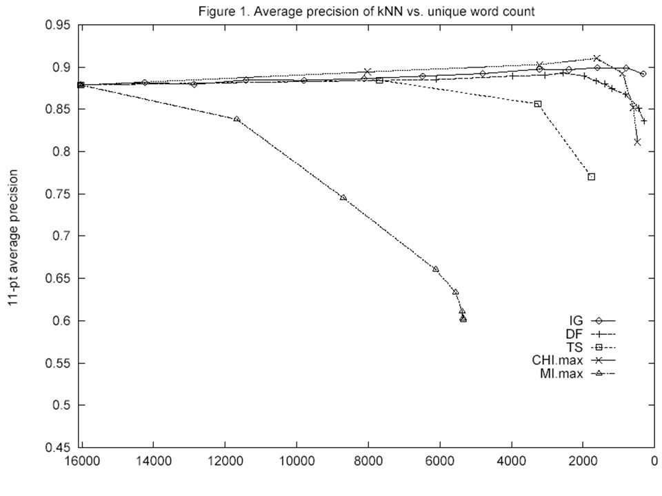
25. Feature Selection Yang and Pedersen 1997 Comparison of different selection criteria – DF – document frequency – IG – information gain – MI – mutual information – CHI – chi square Common strategy – Compute statistic for each term – Keep n terms with highest value of this statistic

26. Feature selection via Mutual Information We might not want to use all words, but just reliable, good discriminators In training set, choose k words which best discriminate the categories. One way is in terms of Mutual Information: – For each word w and each category c

27. (Pointwise) Mutual Information

28. Feature selection via MI (contd.) For each category we build a list of k most discriminating terms. For example (on 20 Newsgroups): – sci.electronics: circuit, voltage, amp, ground, copy, battery, electronics, cooling, … – rec.autos: car, cars, engine, ford, dealer, mustang, oil, collision, autos, tires, toyota, … Greedy: does not account for correlations between terms In general feature selection is necessary for binomial NB, but not for multinomial NB

29. Information Gain

30. Chi-Square Term present Term absent Document belongs to category AB Document does not belong to category CD X^2 = N(AD-BC)^2 / ( (A+B) (A+C) (B+D) (C+D) ) Use either maximum or average X^2 Value for complete independence?

31. Document Frequency Number of documents a term occurs in Is sometimes used for eliminating both very frequent and very infrequent terms How is document frequency measure different from the other 3 measures?

32. Yang&Pedersen: Experiments Two classification methods – kNN (k nearest neighbors; more later) – Linear Least Squares Fit Regression method Collections – Reuters-22173 92 categories 16,000 unique terms – Ohsumed: subset of medline 14,000 categories 72,000 unique terms Ltc term weighting

33. Yang&Pedersen: Experiments Choose feature set size Preprocess collection, discarding non-selected features / words Apply term weighting -> feature vector for each document Train classifier on training set Evaluate classifier on test set

35. Discussion You can eliminate 90% of features for IG, DF, and CHI without decreasing performance. In fact, performance increases with fewer features for IG, DF, and CHI. Mutual information is very sensitive to small counts. IG does best with smallest number of features. Document frequency is close to optimal. By far the simplest feature selection method. Similar results for LLSF (regression).

36. Results Why is selecting common terms a good strategy?

37. IG, DF, CHI Are Correlated.

38. Information Gain vs Mutual Information Information gain is similar to MI for random variables Independence? In contrast, pointwise MI ignores non-occurrence of terms – E.g., for complete dependence, you get: – P(AB)/ (P(A)P(B)) = 1/P(A) – larger for rare terms than for frequent terms Yang&Pedersen: Pointwise MI favors rare terms

39. Feature Selection: Other Considerations Generic vs Class-Specific – Completely generic (class-independent) – Separate feature set for each class – Mixed (a la Yang&Pedersen) Maintainability over time – Is aggressive features selection good or bad for robustness over time? Ideal: Optimal features selected as part of training

40. Yang&Pedersen: Limitations Don’t look at class specific feature selection Don’t look at methods that can’t handle high- dimensional spaces Evaluate category ranking (as opposed to classification accuracy)

41. Feature Selection: Other Methods Stepwise term selection – Forward – Backward – Expensive: need to do n^2 iterations of training Term clustering Dimension reduction: PCA / SVD

42. FEATURES IN SPAM ASSASSIN SpamAssassin is a spam filtering program written in Perl, developed by Justin Mason in 1997 and entirely rewritten by Mark Jeftovic in 2001 when it went on Sourceforge – now maintained by the Apache foundation It uses Naïve Bayes and a variety of other methods It uses features coming both from content and from other properties of the email message

43. 43 SpamAssassin Features 100 From: address is in the user's black-list 4.0 Sender is on www.habeas.com Habeas Infringer List 3.994 Invalid Date: header (timezone does not exist) 3.970 Written in an undesired language 3.910 Listed in Razor2, see http://razor.sf.net/ 3.801 Subject is full of 8-bit characters 3.472 Claims compliance with Senate Bill 1618 3.437 exists:X-Precedence-Ref 3.371 Reverses Aging 3.350 Claims you can be removed from the list 3.284 'Hidden' assets 3.283 Claims to honor removal requests 3.261 Contains "Stop Snoring" 3.251 Received: contains a name with a faked IP-address 3.250 Received via a relay in list.dsbl.org 3.200 Character set indicates a foreign language

44. 44 SpamAssassin Features 3.198 Forged eudoramail.com 'Received:' header found 3.193 Free Investment 3.180 Received via SBLed relay, seehttp://www.spamhaus.org/sbl/ 3.140 Character set doesn't exist 3.123 Dig up Dirt on Friends 3.090 No MX records for the From: domain 3.072 X-Mailer contains malformed Outlook Expressversion 3.044 Stock Disclaimer Statement 3.009 Apparently, NOT Multi Level Marketing 3.005 Bulk email software fingerprint (jpfree) found inheaders 2.991 exists:Complain-To 2.975 Bulk email software fingerprint (VC_IPA) found inheaders 2.968 Invalid Date: year begins with zero 2.932 Mentions Spam law "H.R. 3113" 2.900 Received forged, contains fake AOL relays 2.879 Asks for credit card details

45. 45 Measuring Performance Classification accuracy: What % of messages were classified correctly? Is this what we care about? Overall accuracy Accuracy on spam Accuracy on gen System 195%99.99%90% System 295%90%99.99%  Which system do you prefer?

46. 46 Measuring Performance Precision = good messages kept all messages kept Recall = good messages kept all good messages Trade off precision vs. recall by setting threshold Measure the curve on annotated dev data (or test data) Choose a threshold where user is comfortable

47. 600.465 - Intro to NLP - J. Eisner 47 Measuring Performance low threshold: keep all the good stuff, but a lot of the bad too high threshold: all we keep is good, but we don’t keep much OK for spam filtering and legal search OK for search engines (maybe) would prefer to be here! point where precision=recall (sometimes reported) F-measure = 1 / (average(1/precision, 1/recall))

48. 48 More Complicated Cases of Measuring Performance For multi-way classifiers: – Average accuracy (or precision or recall) of 2-way distinctions: Sports or not, News or not, etc. – Better, estimate the cost of different kinds of errors e.g., how bad is each of the following? – putting Sports articles in the News section – putting Fashion articles in the News section – putting News articles in the Fashion section Now tune system to minimize total cost For ranking systems: – Correlate with human rankings? – Get active feedback from user? – Measure user’s wasted time by tracking clicks? Which articles are most Sports-like? Which articles / webpages most relevant?

49. Micro- vs. Macro-Averaging If we have more than one class, how do we combine multiple performance measures into one quantity? Macroaveraging: Compute performance for each class, then average. Microaveraging: Collect decisions for all classes, compute contingency table, evaluate.

50. Micro- vs. Macro-Averaging: Example Truth: yes Truth: no Classifier: yes 10 Classifier: no 10970 Truth: yes Truth: no Classifier : yes 9010 Classifier : no 10890 Truth : yes Truth: no Classifier: yes 10020 Classifier: no 201860 Class 1Class 2Micro.Av. Table Macroaveraged precision: (0.5 + 0.9)/2 = 0.7 Microaveraged precision: 100/120 =.83 Why this difference?

51. Confusion matrix Function of classifier, topics and test docs. For a perfect classifier, all off-diagonal entries should be zero. For a perfect classifier, if there are n docs in category j than entry (j,j) should be n. Straightforward when there is 1 category per document. Can be extended to n categories per document.

52. 52 Decision Trees Tree with internal nodes labeled by terms Branches are labeled by tests on the weight that the term has Leaves are labeled by categories Classifier categorizes document by descending tree following tests to leaf The label of the leaf node is then assigned to the document Most decision trees are binary trees (never disadvantageous; may require extra internal nodes)

53. 53 Decision Tree Example

54. 54 Decision Tree Learning Learn a sequence of tests on features, typically using top-down, greedy search – At each stage choose unused feature with highest Information Gain (as in Lecture 5) Binary (yes/no) or continuous decisions f1f1 !f 1 f7f7 !f 7 P(class) =.6 P(class) =.9 P(class) =.2

55. Top-down DT induction Partition training examples into good “splits”, based on values of a single “good” feature: (1) Sat, hot, no, casual, keys -> + (2) Mon, cold, snow, casual, no-keys -> - (3) Tue, hot, no, casual, no-keys -> - (4) Tue, cold, rain, casual, no-keys -> - (5) Wed, hot, rain, casual, keys -> +

56. Top-down DT induction keys? yesno Drive: 1,5Walk: 2,3,4

57. Top-down DT induction Partition training examples into good “splits”, based on values of a single “good” feature (1) Sat, hot, no, casual -> + (2) Mon, cold, snow, casual -> - (3) Tue, hot, no, casual -> - (4) Tue, cold, rain, casual -> - (5) Wed, hot, rain, casual -> + No acceptable classification: proceed recursively

58. Top-down DT induction t? coldhot Walk: 2,4 Drive: 1,5 Walk: 3

59. Top-down DT induction t? coldhot Walk: 2,4day? Sat Tue Wed Drive: 1Walk: 3Drive: 5

60. Top-down DT induction t? coldhot Walk: 2,4day? Sat Tue Wed Drive: 1Walk: 3Drive: 5 Mo, Thu, Fr, Su ? Drive

61. Top-down DT induction: divide and conquer algorithm Pick a feature Split your examples into subsets based on the values of the feature For each subsets, examine the examples: – Zero: assign the most popular class for the parent – All from the same class: assign this class – Otherwise, process recursively

62. Top-Down DT induction Different trees can be built for the same data, depending on the order of features: t? coldhot Walk: 2,4day? Sat Tue We d Drive: 1Walk: 3Drive: 5 Mo, Thu, Fr, Su ? Drive

63. Top-down DT induction Different trees can be built for the same data, depending on the order of features: t? coldhot Walk: 2,4day? Sat Tue We d Drive: 1Walk: 3Drive: 5 Mo Drive:? clothing casual halloween walk:?

64. Selecting features Intuitively – We want more “informative” features to be higher in the tree: Is it Monday? Is it raining? Good political news? No halloween cloths? Hat on? Coat on? Car keys? Yes?? -> Driving! (doesn't look as a good learning job) – We want a nice compact tree..

65. Selecting features-2 Formally – Define “tree size” (number of nodes, leaves; depth,..) – Try all the possible trees, find the smallest one – NP-hard Top-down DT induction – greedy search, depends on heuristics for feature ordering (=> no guarantee) – Information gain

66. Entropy Information theory: entropy – number of bits needed to encode some information. S – set of N examples: p*N positive (“Walk”) and q*N negative (“Drive”) Entropy(S)= -p*lg(p) – q*lg(q) p=1, q=0 => Entropy(S)=0 p=1/2, q=1/2 => Entropy(S)=1

67. Entropy and Decision Trees keys? noyes Walk: 2,4Drive: 1,3,5 E(S)=-0.6*lg(0.6)-0.4*lg(0.4)= 0.97 E(Sno)=0E(Skeys)=0

68. Entropy and Decision Trees t? coldhot Walk: 2,4 Drive: 1,5 Walk: 3 E(S)=-0.6*lg(0.6)-0.4*lg(0.4)= 0.97 E(Scold)=0E(Shot)=-0.33*lg(0.33)-0.66*lg(0.66)= 0.92

69. Information gain For each feature f, compute the reduction in entropy on the split: Gain(S,f)=E(S)- ∑(Entropy(Si)* |Si|/|S|) f=keys? : Gain(S,f)=0.97 f=t?: Gain(S,f)=0.97-0*2/5-0.92*3/5=0.42 f=clothing?: Gain(S,f)= ?

70. TEXT CATEGORIZATION WITH DT Build a separate decision tree for each category Use WORDS COUNTS as features

71. 71 Reuters Data Set ( 21578 - ModApte split) 9603 training, 3299 test articles; ave. 200 words 118 categories – An article can be in more than one category – Learn 118 binary category distinctions Earn (2877, 1087) Acquisitions (1650, 179) Money-fx (538, 179) Grain (433, 149) Crude (389, 189) Trade (369,119) Interest (347, 131) Ship (197, 89) Wheat (212, 71) Corn (182, 56) Common categories (#train, #test)

72. Foundations of Statistical Natural Language Processing, Manning and Schuetze AN EXAMPLE OF REUTERS TEXT

73. Foundations of Statistical Natural Language Processing, Manning and Schuetze Decision Tree for Reuter classification

74. Conquer-and-divide with Information gain Batch learning (read all the input data, compute information gain based on all the examples simultaneously) Greedy search, may find local optima Outputs a single solution Optimizes depth

75. Complexity Worst case: build a complete tree – Compute gains on all nodes: at level i, we have already examined i features; m-i remaining. In practice: tree is rarely complete, linear on number of features, number of examples (== very fast)

76. Overfitting Suppose we build a very complex tree.. Is it good? Last lecture: we measure the quality (“goodness”) of the prediction, not the performance on the training data Why can complex trees yield mistakes: – Noise in the data – Even without noise, solutions at the last levels are based on too few observations

77. Overfitting Mo: Walk (50 observations), Drive (5) Tue: Walk (40), Drive (3) We: Drive (1) Thu: Walk (42), Drive (14) Fri: Walk (50) Sa: Drive (20), Walk (20) Su: Drive (10) Can we conclude that “We->Drive”?

78. Overfitting A hypothesis H is said to overfit the training data if there exist another hypothesis H' such that: Error(H, train data) <= Error (H', train data) Error(H, unseen data) > Error (H', unseen data) Overfitting is related to hypothesis complexity: a more complex hypothesis (e.g., a larger decision tree) overfits more

79. Overfitting Prevention for DT: Pruning “prune” a complex tree: produce a smaller tree that is less accurate on the training data Original tree:...Mo: hot->drive (2), cold -> walk (100) Pruned tree:.. Mo-> walk (100/2) post-/pre- pruning

80. Pruning criteria Cross-validation – Reserve some training data to evaluate the utility of the subtrees Statistical tests: use a test to determine whether observations at given level can be random MDL (minimum description length): compare the added complexity against memorizing exceptions

81. DT: issues Splitting criteria – Information gain: split at features with many values Non-discrete features Non-discrete outputs (“regression trees”) Costs Missing values Incremental learning Memory issues

82. REFERENCES Tom Mitchell, Machine Learning. McGraw- Hill, 1997. – Chapter 6, Bayesian Learning - 6.1, 6.2, 6.9, 6.10 – Chapter 3, Decision Trees – whole chapter Fabrizio Sebastiani. Machine Learning in Automated Text Categorization. ACM Computing Surveys, 34(1):1-47, 2002

83. ACKNOWLEDGMENTS Many slides borrowed from Chris Manning, Stanford