Download presentation
Presentation is loading. Please wait.

2
C. Models 1. Pathogens

3
C. Models 1. Pathogens R = (b/g)S b = rate of transmission g = recovery time (inverse of infectious period)
S b = rate of transmission g = recovery time (inverse of infectious period).")
4
C. Models 2. Lotka-Volterra Models Goal - create a model system in which there are oscillations of predator and prey populations that are out-of-phase with one another. Basic Equations: a. Prey Equation: dV/dt = rV - cVP where rV defines the maximal, geometric rate c = predator foraging efficiency: % eaten P = number of predators V= number of prey, so PV = number of encounters and cPV = number of prey killed (consumed) So, the formula describes the maximal growth rate, minus the number of prey individuals lost by predation.
 So, the formula describes the maximal growth rate, minus the number of prey individuals lost by predation..")
5
Number of Prey (V)
")
6
C. Models 2. Lotka-Volterra Models b. Predator The Equation: dP/dt = a(cPV) - dP where CPV equals the number of prey consumed, and a = the rate at which food energy is converted to offspring. So, a(cVP) = number of predator offspring produced. d = mortality rate, and P = # of predators, so dP = number of carnivores dying. So, the equation boils down to the birth rate (determined by energy "in" and conversion rate to offspring) minus the death rate.
 - dP where CPV equals the number of prey consumed, and a = the rate at which food energy is converted to offspring. So, a(cVP) = number of predator offspring produced. d = mortality rate, and P = # of predators, so dP = number of carnivores dying. So, the equation boils down to the birth rate (determined by energy in and conversion rate to offspring) minus the death rate..")
8
Basic Equations: 1. Prey 2. Predator 3. Dynamics 1. 2.3. 4. 1.2.3.4.1.

11
V. Dynamics of Consumer-Resource Interactions A. Predators can limit the growth of prey populations B. Oscillations are a Common Pattern C. Models D. Lab Experiments 1. Gause P. caudatum (prey) and Didinium nasutum (predator)
 and Didinium nasutum (predator).")
12
In initial experiments, Paramecium populations would increase, followed by a pulse of Didinium, and then they would crash.

13
P. caudatum (prey) and Didinium nasutum (predator) In initial experiments, Paramecium populations would increase, followed by a pulse of Didinium, and then they would crash. He added glass wool to the bottom, creating a REFUGE that the predator did not enter.
 and Didinium nasutum (predator) In initial experiments, Paramecium populations would increase, followed by a pulse of Didinium, and then they would crash. He added glass wool to the bottom, creating a REFUGE that the predator did not enter..")
14
He induced oscillations by adding Paramecium as 'immigrants'

15
D. Laboratory Experiments 1. Gause 2. Huffaker six-spotted mite (Eotetranychus sexmaculatus) was prey - SSM Predatory mite (Typhlodromus occidentalis) was predator - PM
 was prey - SSM Predatory mite (Typhlodromus occidentalis) was predator - PM.")
18
D. Laboratory Experiments 1. Gause 2. Huffaker 3. Holyoak and Lawler-1996

19
Holyoak and Lawler-1996 Used a bacteriovore ciliate, Colpidium striatum as the prey and our old friend Didinium nasutum as the predator.

20
3. Holyoak and Lawler-1996 Set up replicate 30mL bottles, linked together by tubes, and single flask systems.

21
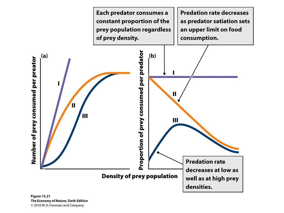
D. Complexities and Applications 2. Multiple State States Consider a Type III functional response, where the predation rate is highest at intermediate prey densities. V Birth rate Predation Rate

22
D. Complexities and Applications 2. Multiple State States Consider a Type III functional response, where the predation rate is highest at intermediate prey densities. V Birth rate Predation Rate

Similar presentations


 Predator-prey cycles Models of predation>")


