1. Persistence of forage fish ‘hot spots’ and its association with foraging Steller sea lions in southeast Alaska Scott M. Gende National Park Service, Glacier Bay Field Station, 3100 National Park, Juneau, Alaska, USA; Scott_Gende@nps.gov Michael F. Sigler National Marine Fisheries Service, Alaska Fisheries Science Center, Auke Bay Laboratory, Juneau, Alaska, USA; Mike.Sigler@noaa.gov

3. 1. 1. Identify aggregations of pelagic fish prey in space and time. 2. 2.Examine whether these prey ‘hot spots’ persist within and across seasons. 3. 3.Examine which characteristics of prey aggregations are associated with predator aggregations. 4. 4.Model foraging effort (efficiency) as it varies with these characteristics. Objectives:

4. Upper Lynn canal, southeast Alaska ~40 linear km

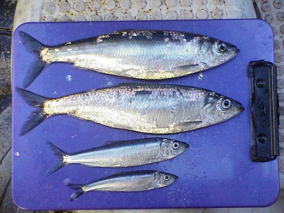
5. Methods: 1. Hydroacoustic surveys for pelagic prey conducted June 2001-May 2004 2. Periodic midwater trawls to sample prey energy and confirm echo sound 3. Concurrent observations of top predators including Steller sea lions and humpback whales 4. Transformed data from estimates of biomass to energy densities integrated across the water column 5. Blocked data into tenths of a latitudinal minute such that each ‘block’ constituted approximately 1.83 km)

6. Methods: 1. Hydroacoustic surveys for pelagic prey conducted June 2001-May 2004 2. Periodic midwater trawls to sample prey energy and confirm echo sound 3. Concurrent observations of top predators including Steller sea lions and humpback whales 4. Transformed data from estimates of biomass to energy densities integrated across the water column 5. Blocked data into tenths of a latitudinal minute such that each ‘block’ constituted approximately 1.83 km)

7. Methods: 1. Hydroacoustic surveys for pelagic prey conducted June 2001-May 2004 2. Periodic midwater trawls to sample prey energy and confirm echo sound 3. Concurrent observations of top predators including Steller sea lions and humpback whales 4. Transformed data from estimates of biomass to energy densities integrated across the water column 5. Blocked data into tenths of a latitudinal minute such that each ‘block’ constituted approximately 1.83 km)

8. Methods: 1. Hydroacoustic surveys for pelagic prey conducted June 2001-May 2004 2. Periodic midwater trawls to sample prey energy and confirm echo sound 3. Concurrent observations of top predators including Steller sea lions and humpback whales 4. Blocked data into tenths of a latitudinal minute such that each ‘block’ constituted approximately 1.83 km 5. Transformed data from estimates of biomass to energy densities integrated across the water column

9. Methods: 1. Hydroacoustic surveys for pelagic prey conducted June 2001-May 2004 2. Periodic midwater trawls to sample prey energy and confirm echo sound 3. Concurrent observations of top predators including Steller sea lions and humpback whales 5. Transformed data from estimates of biomass to energy densities integrated across the water column kJ x 10 6 /km 2 4. Blocked data into tenths of a latitudinal minute such that each ‘block’ constituted approximately 1.83 km)

10. Results:

11. Strong seasonal variation in prey energy density; consistent across three years Average energy density in study area (Millions kJ/km 2) 20012004

12. Cold winter months (Nov-Feb) are hot Average energy density in study area (Millions kJ/km 2) 20012004

15. Seasonal haul-out > 20000 10000-20000 5000-10000 1000-5000 1-1000 Prey energy density and SSL locations: Nov 03 >70% 50-70% 30-50% 10-30% <10% Prey energy % of SSL

16. Seasonal haul-out > 20000 10000-20000 5000-10000 1000-5000 1-1000 Prey energy density and SSL locations: Dec 03 >70% 50-70% 30-50% 10-30% <10% Prey energy % of SSL

17. Seasonal haul-out > 20000 10000-20000 5000-10000 1000-5000 1-1000 Prey energy density and SSL locations: Jan 04 >70% 50-70% 30-50% 10-30% <10% Prey energy % of SSL

18. Seasonal haul-out > 20000 10000-20000 5000-10000 1000-5000 1-1000 Prey energy density and SSL locations: Feb 04 >70% 50-70% 30-50% 10-30% <10% Prey energy % of SSL

19. Seasonal haul-out > 20000 10000-20000 5000-10000 1000-5000 1-1000 Prey energy density and SSL locations: Mar 04 >70% 50-70% 30-50% 10-30% <10% Prey energy % of SSL

20. Seasonal haul-out > 20000 10000-20000 5000-10000 1000-5000 1-1000 Prey energy density and SSL locations: Apr 04 >70% 50-70% 30-50% 10-30% <10% Prey energy % of SSL

21. Seasonal haul-out > 20000 10000-20000 5000-10000 1000-5000 1-1000 Prey energy density and SSL locations: May 04 >70% 50-70% 30-50% 10-30% <10% Prey energy % of SSL

22. Seasonal haul-out Proportion of surveys where above average prey densities were located: winter months (Nov-Feb) >70% 60-70% 50-60%

23. Seasonal haul-out >70% 60-70% 50-60% 20-30% Proportion of surveys where above average prey densities were located: non-winter months (Mar-Oct)

24. Seasonal haul-out Prey persistence relative to locations of foraging sea lions: winter >70% 60-70% 50-60% Prey persistence >40% 30-40% 20-30% Foraging SSL

25. Persistence (Proportion of surveys patch was hot) Proportion of months sea lions found foraging within patch Winter: R 2 = 0.41 Non-winter: R 2 = 0.01

26. Proportion of months sea lions found foraging within patch Persistence: R 2 = 0.41 Average Density (Proportion of surveys patch was hot) Density: R 2 = 0.36

27. 1. Are prey aggregated in time and space? Overwintering herring schools result in high prey aggregations Nov-Feb and occur in consistent locations.Overwintering herring schools result in high prey aggregations Nov-Feb and occur in consistent locations. 2. Do these prey ‘hot spots’ persist? The probability of encountering a high concentration of prey exceeded 70% for some areasThe probability of encountering a high concentration of prey exceeded 70% for some areas 3.Do predators respond to this persistence? Strong relationship (during the winter) between sea lion distribution and distribution of prey. However, it appears that sea lion’s response is strongest in areas with highest prey persistence, not necessarily highest densityStrong relationship (during the winter) between sea lion distribution and distribution of prey. However, it appears that sea lion’s response is strongest in areas with highest prey persistence, not necessarily highest density

28. So what?

29. A foraging effort model: How will foraging effort of sea lions vary with density or persistence of prey hot spots?

30. xxx T1T1T1T1 T2T2T2T2 T3T3T3T3....T 10 Prey distribution: High density, low persistence xxx Low density, low persistence Low density, low persistence xxx Low density, high persistence Low density, high persistence

31. PersistenceLowHigh Foraging Effort Prey density = High Random walk Bayesian forager Prey density = Mid Persistence LowHigh Persistence LowHigh Prey density = Low

32. Density may not be the only characteristic of prey aggregations that are important to predators; persistence may be just as important, particularly for those that do not have the ability to search large areas efficiently.

33. Special thanks to : Dave Csepp, JJ Volldenweider, and Jamie Womble. This project funded by the Auke Bay Laboratory, National Marine Fisheries Service