Tamara Berg CS Artificial Intelligence

Tamara Berg CS 590-133 Artificial Intelligence
Search Tamara Berg CS Artificial Intelligence Course is modeled after similar courses at UC Berkeley, UIUC, University of Washington and elsewhere. Many slides throughout the course will be adapted from these people. Many slides throughout the course adapted from Dan Klein, Stuart Russell, Andrew Moore, Svetlana Lazebnik, Percy Liang, Luke Zettlemoyer

Course Information Instructor: Tamara Berg Course website: TAs: Shubham Gupta & Rohit Gupta Office Hours (Tamara): Tuesdays/Thursdays 4:45-5:45pm FB 236 Office Hours (Shubham): Mondays 4-5pm & Friday 3-4pm SN 307 Office Hours (Rohit): Wednesday 4-5pm & Friday 4-5pm SN 312 Ok this is the last time I’m putting this up in case there are any new students today See website & previous slides for additional important course information.

Announcements for today
Sign up for the class piazza mailing list here: piazza.com/unc/spring2014/comp590133 Reminder: This is a 3 credit course. If you are enrolled for 1 credit, please change to 3 credits. HW1 will be released on the course website tonight (Shubham/Rohit will give a short overview at the end of class)

Recall from last class

Agents An agent is anything that can be viewed as perceiving its environment through sensors and acting upon that environment through actuators An agent is anything that can be viewed as perceiving its environment through sensors and acting upon that environment through actuators. Can you think of any potential agents? Human is an agent. Sensors are eyes, ears, mouth, actuators are arms, limbs, vocal tract that we use to act on the environment. Robot agent. Sensors =cameras, range finders, etc. actuators = motors Software agent. Sensors=keystrokes, network packets. Actuators = display on screen, write files, etc. An agent function maps any given percept sequence to an action.

Rational agents For each possible percept sequence, a rational agent should select an action that is expected to maximize its performance measure, given the evidence provided by the percept sequence and the agent’s built-in knowledge Performance measure (utility function): An objective criterion for success of an agent's behavior In this class we’ll talk a lot about rational agents. We define a rational agent as one who does the right thing, but what is the right thing? Well let’s say you plunk the agent down in the environment and it generates actions according to its percepts. If the action sequence is desirable, then the agent has performed well. -> more concretely a rational agent should select an action that is expected to maximize its performance measure given the evidence provided by the percept sequence and the agent’s built-in knowledge. So we need some performance measure (also called a utility function) that evaluates the goodness of a sequence of actions and their resulting environment states. Then a rational agent should act to maximize it’s expected utility. How do we calculate expected the utility of an action? ExpectedUtility(action) = sum_outcomes Utility(outcome) * P(outcome|action)

Types of agents Reflex agent Planning agent Consider how the world IS
Choose action based on current percept (and maybe memory or a model of the world’s current state) Do not consider the future consequences of their actions Consider how the world WOULD BE Decisions based on (hypothesized) consequences of actions Must have a model of how the world evolves in response to actions Must formulate a goal (test) There are different types of agents. A reflex agent considers how the world currently is, and chooses an action based on their current percept (and maybe memory or a model of the world’s state). They do not consider the future consequences of their actions, they just react to the world with actions. One example is our simple vacuum agent. In the vacuum world, if there’s dirt then the vaccum sucks, if they are in square A then they move to square B. the vacuum agent doesn’t plan ahead. Goal or planning based agents plan ahead, they ask what if and consider how the world would be if they executed an action. Their decisions are based on (hypothesized) consequences of actions. They need a model of how the world evolves in response to actions and formulate a goal (with a corresponding goal test). Goals help organize an agent’s behavior by limiting the objectives an agent is trying to achieve and hence the actions it needs to consider.

Search We will consider the problem of designing goal-based agents in fully observable, deterministic, discrete, known environments Start state We will consider the problem of designing goal-based agents in fully observable, deterministic, discrete, known environments. Goal state

Search problem components
Initial state Actions Transition model What state results from performing a given action in a given state? Goal state Path cost Assume that it is a sum of nonnegative step costs The optimal solution is the sequence of actions that gives the lowest path cost for reaching the goal Initial state So to formulate a problem like this we need to define a number of things. The initial state – the state that the agent starts in The actions – available to the agent, Actions(s) given a particular state s The transition model – this is a description of what each action does. Result(s,a) returns the state that restults from doing action a in state s. The goal state determines whether a given state is a goal state For any sequence of actions we can calculate their cost – the path cost - where we assume that the cost of a path is the sum of costs of individual actions and each action has non-negative cost. The optimal solution to the search problem is a sequence of actions that gives the lowest path cost for reaching the goal. Goal state

Example: Romania On vacation in Romania; currently in Arad
Flight leaves tomorrow from Bucharest Initial state Arad Actions Go from one city to another Transition model If you go from city A to city B, you end up in city B Goal state Bucharest Path cost Sum of edge costs (total distance traveled) Let’s make it more concrete with an example. Let’s say our agent is on vacation in romania, currently in arad. He has a flight that leaves tomorrow from bucharest. So he needs to get to bucharest by tomorrow. What is the initial state? In(Arad) What are the possible actions the agent can take – drive from one city to another. If in arad, he can drive to zerind or timisoara. If in timisoara he can drive to lugo or arad and so on. What is the transition model? If you drive from city to A to city B you end up in city B so result(In(arad),go(zerind)) = in(zerind) What is the goal state: being In(bucharest) What might be the path cost – sum of edge costs (total distance traveled along any path). So cost of In(arind),go(zerind),in(zerind) = 75

State space The initial state, actions, and transition model define the state space of the problem The set of all states reachable from initial state by any sequence of actions Can be represented as a directed graph where the nodes are states and links between nodes are actions We can also talk about the state space of our problem. This is the set of all states of the world reachable from the initial state by any sequence of actions. This can be represented as a directed graph where the nodes are states and links between nodes are actions.

Vacuum world state space graph
Here is the state space of vacuum world. Each of the nodes is a possible state of the world, and arcs between states represent transitions by actions. So if we are in the leftmost state and we execute the action left, then nothing happens (because we’re already in the left square) and we remain in the same state. Same for suck. But if we execute the action move(right) then we end up in the next state over. This is a tiny state space because our world is really simple.

Search Given: How do we find the optimal solution?
Initial state Actions Transition model Goal state Path cost How do we find the optimal solution? How about building the state space and then using Dijkstra’s shortest path algorithm? Complexity of Dijkstra’s is O(E + V log V), where V is the size of the state space The state space may be huge! In search we are given an initial state, possible actions that you can make from each state, a transition model that tells you given that you are in state s and take action a what state will you be in next. A goal state or states and a path cost function. How could we find the optimal solution? Well some of you might say why don’t we build the state space and then use a shortest path algorithm to find the shortest path from the initial state to the goal. Great! But the complexity of doing this is on the order of E+VlogV where V is the size of the state space and the state space may be huge!!!

Search: Basic idea Let’s begin at the start state and expand it by making a list of all possible successor states Maintain a frontier – the set of all leaf nodes available for expansion at any point At each step, pick a state from the frontier to expand Keep going until you reach a goal state or there are no more states to explore. Try to expand as few states as possible So instead we will use search to find a solution. An agent with several intermediate actions of unknown value can decide what to do by first examining future actions that eventually lead to states of known value (e.g. a goal state). The agent can find a path through the state space (a sequence of actions) that reaches a goal state and then it can execute those actions. They can find this sequence of actions using search. The basic idea of searching will be that we’ll begin at the start state and expand it by making a list of all possible successor states. We will maintain a frontier, or list of unexpanded states that we might want to explore next. And at each step, we’ll pick a state from the frontier to expand (this will put new states on the frontier list) and so on until we reach a goal state. Ideally we want to expand as few states as possible to reach the goal.

… Search tree “What if” tree of sequences of actions and outcomes
The root node corresponds to the starting state The children of a node correspond to the successor states of that node’s state A path through the tree corresponds to a sequence of actions A solution is a path ending in a goal state Edges are labeled with actions and costs … Starting state Successor state Action Goal state A search tree is essentially a “what if” tree of sequences of actions and outcomes, with the starting state at the root. the children of a node correspond to the successor states of that node’s state (states that are reachable through an action). A path through this tree corresponds to a sequence of actions (so for any node there is some corresponding set of actions that takes you from the start state to that state). A solution is a path ending in a goal state. Edges are labeled with actions and costs.

So for this example state graph what does the search tree look like?

S (the start state) is at the root, it’s successors (aka children that can be reached via some action) are d,e,p so those are the next level of the tree. Each of those has children d’s children are b,c,e so those are below d in the tree and so on. Each node in the search tree is an entire path in the state graph. A solution – for example the one in red – is a path ending in the goal state, so here the path is s->d->e->r->f->g (a path that starts in the start state and ends in the goal state).

Tree Search Algorithm Outline
Initialize the frontier using the start state While the frontier is not empty Choose a frontier node to expand according to search strategy and take it off the frontier If the node contains the goal state, return solution Else expand the node and add its children to the frontier We will use tree search to find solutions to our search problems. Here is an outline of the tree search algorithm: We initialize the frontier set using the start state. Then while the frontier set is not empty: choose a frontier node to expand according to your search strategy and take it off the frontier if the node contains a goal state, return the solution else expand the node (according to the state’s possible actions) and add its children to the frontier set We’ll talk about specific search strategies next class. For now, imagine some black box just decides which frontier node to expand next.

Tree search example Start: Arad Goal: Bucharest
Let’s look at tree search for our romania problem. What do we do first? Set the frontier to arad (the start state). Note, we will denote what’s on the frontier list as white, and things not currently on the frontier list as grey. What do we do next? We choose a frontier state to be expanded. So we choose arad and expand it. Well possible actions from arad are driving to zerind, timisoara or sibiu. Start: Arad Goal: Bucharest

So we add those to our frontier list. Now we need to choose another state from our frontier list to expand. Let’s say we choose sibiu. Start: Arad Goal: Bucharest

We expand sibiu – from sibiu you can go to arad, fageras, oradea or RV so we add those to our frontiers list. Next let’s say we choose RV. Start: Arad Goal: Bucharest

We take RV off the frontiers list, and expand it to it’s successors – craiova, pitesti, and sibiu. Maybe next we choose fageras from our frontiers list Start: Arad Goal: Bucharest

Take it off and add its successors. Then we choose pitesti. Start: Arad Goal: Bucharest

Take it off and add it’s successors. Start: Arad Goal: Bucharest

Pitesti has bucharest as a successor, so we’ve reached our goal. Woohoo!!! Did you notice anything odd about this search tree? Where is arad? Top and later. So we have some repeated states that we might accidentally explore multiple times… Start: Arad Goal: Bucharest

Handling repeated states
Initialize the frontier using the starting state While the frontier is not empty Choose a frontier node to expand according to search strategy and take it off the frontier If the node contains the goal state, return solution Else expand the node and add its children to the frontier To handle repeated states: Keep an explored set; which remembers every expanded node Newly generated nodes already in the explored set or frontier can be discarded instead of added to the frontier One way to handle repeated states is to keep an additional set besides the frontier, an explored set. We add each node to the explored set when we expand it. Everytime you add a node to the frontier, check whether it already exists in the frontier with a higher path cost, and if yes replace that node with the new one.

Search without repeated states
Now we start of the same way in arad. We expand it and put it’s successors on the frontiers list. Start: Arad Goal: Bucharest

We expand sibiu Start: Arad Goal: Bucharest

It’s successors include arad. In this case, arad has a higher path cost than the previous arad in the explored set, so we can discard this node (ie not add it to the frontier list). Start: Arad Goal: Bucharest

We expand RV. It has a successor sibiu whose path cost is larger than the previously explored sibiu, so we can discard this node. Start: Arad Goal: Bucharest

And so on Start: Arad Goal: Bucharest

… Start: Arad Goal: Bucharest

… until we reach the goal. This lets us search without getting stuck in loops by remembering where we’ve been already. Start: Arad Goal: Bucharest

Tree Search Algorithm Outline
Initialize the frontier using the starting state While the frontier is not empty Choose a frontier node to expand according to search strategy and take it off the frontier If the node contains the goal state, return solution Else expand the node and add its children to the frontier Main question: What should our search strategy be, ie how do we choose which frontier node to expand? Ok so back to the basic tree search algorithm. What is the main thing we have to define here? What search strategy should we use – ie how should we decide which frontier node to expand.

Uninformed search strategies
A search strategy is defined by picking the order of node expansion Uninformed search strategies use only the information available in the problem definition Breadth-first search Depth-first search Iterative deepening search Uniform-cost search A search strategy is defined by picking the order of node expansion. We’ll talk about two different types of search strategies, uninformed and informed search. Uninformed search strategies use only the information available in the problem definition. So, there is no additional information about states. We can just generate successors and test for the goal state. Examples include BFS, DFS, Iterative deepening, and uniform-cost search

Informed search strategies
Idea: give the algorithm “hints” about the desirability of different states Use an evaluation function to rank nodes and select the most promising one for expansion Greedy best-first search A* search Search strategies that know whether one non-goal state is “more promising” than another are called informed or heuristic search. These strategies use an evaluation function to rank nodes and select the most promising one for expansion. The main idea of these kinds of strategies is that the evaluation function gives the algorithm “hints” about the desirability of different states. Examples of this that we’ll look at include greedy best-first search and A* search.

Uninformed search Let’s first look at examples of uninformed search.

Example state space graph for a tiny search problem
Breadth-first search Expand shallowest node in the frontier Example state space graph for a tiny search problem You’ve probably all seen breadth-first search before. Q: What is the search strategy here? BFS expands the shallowest unexpanded node. Let’s look at an example. Here is an example state space for a tiny search problem where we start at state s and want to get to state g. Example from P. Abbeel and D. Klein

Breadth-first search Expansion order: (S,d,e,p,b,c,e,h,r,q,a,a, h,r,p,q,f,p,q,f,q,c,G) So what do we do first? We put s on the frontier. Then while the frontier is not empty we take the shallowest node off the frontier (in this case it’s s because that’s the only node on the frontier). We expand s and put it’s children on the frontier – d,e,p. now which node do we expand next?

Breadth-first search Expansion order: (S,d,e,p,b,c,e,h,r,q,a,a, h,r,p,q,f,p,q,f,q,c,G) d because d,e,p are on the frontier and d is the shallowest node on the frontier. So we take off d. it’s not the goal so we put on it’s children, b,c,e. What node do we expand next?

Breadth-first search Expansion order: (S,d,e,p,b,c,e,h,r,q,a,a, h,r,p,q,f,p,q,f,q,c,G) E because it’s the shallowest node on the frontier. So we take e off. It’s not a goal state so we add it’s children to the frontier h,r. which node is next?

Breadth-first search Expansion order: (S,d,e,p,b,c,e,h,r,q,a,a, h,r,p,q,f,p,q,f,q,c,G) p. next?

Breadth-first search Expansion order: (S,d,e,p,b,c,e,h,r,q,a,a, h,r,p,q,f,p,q,f,q,c,G) And so on. Until we reach the goal state. 23 nodes expanded.

Example state space graph for a tiny search problem
Breadth-first search Expand shallowest node in the frontier Implementation: frontier is a FIFO queue Example state space graph for a tiny search problem Q: so how do you implement this kind of frontier? With a FIFO queue (the shallowest node was added first to the queue, therefore it is the first thing taken off) Example from P. Abbeel and D. Klein

Depth-first search Expand deepest node in the frontier
Depth first search is similar, except instead of expanding the shallowest node, DFS expands the deepest node in the frontier. So for that same state space graph the expansion ordering is quite different.

Depth-first search Expansion order: (S,d,b,a,c,a,e,h,p,q,q, r,f,c,a,G)

Depth-first search Expansion order: (S,d,b,a,c,a,e,h,p,q,q,r,f,c,a,G)
And so on until we reach the goal state. (16 nodes expanded)

Depth-first search Expand deepest unexpanded node
Implementation: frontier is a LIFO queue Q: How do we implement DFS frontier? With a LIFO queue so that the last thing put into the queue is expanded first (the deepest node has been added last therefore it gets expanded first)

Analysis of search strategies
Strategies are evaluated along the following criteria: Completeness does it always find a solution if one exists? Optimality does it always find a least-cost solution? Time complexity how long does it take to find a solution? Space complexity maximum number of nodes in memory Time and space complexity are measured in terms of b: maximum branching factor of the search tree d: depth of the optimal solution m: maximum length of any path in the state space (may be infinite) We can evaluate search strategies with different criteria.

Properties of breadth-first search
Complete? Yes (if branching factor b is finite) Optimal? Not generally – the shallowest goal node is not necessarily the optimal one Yes – if all actions have same cost Time? Number of nodes in a b-ary tree of depth d: O(bd) (d is the depth of the optimal solution) Space? O(bd) Is BFS search complete? Yes BFS will eventually find the shallowest goal node after generating all shallower nodes (if the branching factor is not infinite). Is BFS optimal? Not generally because the shallowest goal node is not necessarily the optimal one. However in some cases bfs is optimal, for example, if all actions have the same cost. Ok, so that’s pretty good. What about time? Imagine searching a uniform tree where every state has b successors. The root of the tree generates b nodes at the first level, each of which generates b more nodes (so b^2 at the second level), each of these generates b more nodes, so b^3 at the third level and so on. If the solution is at depth d, then the total number of nodes generated is b+b^2+b^3+b^4…+b^d = O(b^d). How about space? Well think about the last level, there will be O(b^d) nodes in the frontier. So the space complexity is O(b^d).

BFS Depth Nodes Time Memory 2 110 0.11 ms 107 kilobytes 4 11,110 11 ms 10.6 megabytes 6 10^6 1.1 s 1 gigabyte 8 10^8 2 min 103 gigabytes 10 10^10 3 hrs 10 terabytes 12 10^12 13 days 1 petabyte 14 10^14 3.5 years 99 petabytes 16 10^16 350 years 10 exabytes In general space is the bigger problem (more than time). You might be able to wait 13 days for the solution to an important problem with search depth 12, but no personal computer has the petabyte of memory that it would take. Of course time is still a major factor too. If your problem has a solution at depth 16, it will take about 350 years for BFS to find it! Time and Space requirements for BFS with b=10; 1 million nodes/second; 1000 bytes/node

Properties of depth-first search
Complete? Fails in infinite-depth spaces, spaces with loops Modify to avoid repeated states along path  complete in finite spaces Optimal? No – returns the first solution it finds Time? May generate all of the O(bm) nodes, m=max depth of any node Terrible if m is much larger than d Space? O(bm), i.e., linear space! What about depth first search? Complete? Well the basic tree search algorithm obviously fails in infinite-depth spaces or spaces with loops. If we modify the algorithm to avoid repeated states along the path then it is complete in finite state spaces. Optimal? No, dfs simply returns the first solution it finds, which may not be the optimal one. Time? Tree search for DFS may generate all of the O(b^m) nodes in the search tree, where m is the maximum depth of any node. M itself can be much larger than d (the depth of the shallowest solution). So why do we care about DFS? The reason is space complexity. For tree search DFS (without handling repeated states), DFS needs to store only a single path from the root to a leaf node, along with the remaining unexpanded sibling nodes for each node on the path. For state space with branching factor b and max depth m, depth first search requires storage of only O(bm) nodes! For this reason, DFS is used in a lot of problems in AI.

Iterative deepening search
Use DFS as a subroutine Check the root Do a DFS with depth limit 1 If there is no path of length 1, do a DFS search with depth limit 2 If there is no path of length 2, do a DFS with depth limit 3. And so on… The failure of DFS in infinite state spaces can be alleviated by supplying it with a pre-determined depth limit, l. depth are treated as if they have no successors. This is good, because you won’t get stuck going down an infinite path. Why might it be bad? Will not be complete if l < d. The solution is iterative deepening search. This essentially gradually increases the value for l until a goal is found. This algorithm uses DFS as a subroutine. First check whether the root is the goal. Else do a DFS with depth limit 1, if there is no path of length 1 do a DFS with depth limit 2. If there is no path of length 2, do a DFS with depth limit 3. and so on

Here’s what that looks like. We first check whether the root is a goal node.

Then we do DFS with limit 1.

Then with limit 2

Limit 3 and so on until we reach a goal.

Properties of iterative deepening search
Complete? Yes Optimal? Not generally – the shallowest goal node is not necessarily the optimal one Yes – if all actions have same cost Time? (d+1)b0 + d b1 + (d-1)b2 + … + bd = O(bd) Space? O(bd) What is this doing at a high level? Essentially it is combining the benefits of BFS and DFS, giving a modest memory requirement, and compleness when b is finite. Is it complete? Yes when b is finite. Optimal? Similarly to BFS it’s optimal when all actions have the same cost Time? Seems like this is where you would pay – because states are generated multiple times, but it turns out this is not too costly because in a search tree with the same (or nearly the same) branching factor at each level, most of the nodes are in the bottom level. So, it doesn’t matter much that the upper levels are generated multiple times. Space? Is the same as DFS.

Search with varying step costs
One problem that we saw with BFS is that it finds the path with the fewest steps, but that might not always be the lowest cost path. This path has the fewest steps to the goal, but is cost = 14. this other path S->d->e->r->f->G has more steps, but it’s cost is = 10 which has lower cost. BFS finds the path with the fewest steps, but does not always find the cheapest path

Uniform-cost search For each frontier node, save the total cost of the path from the initial state to that node Expand the frontier node with the lowest path cost Implementation: frontier is a priority queue ordered by path cost Equivalent to breadth-first if step costs all equal One simple solution to this is uniform cost search. For each frontier node, we save the total cost of the path from the initial state to that node. Now when we select a node to expand instead of choosing the shallowest node, we select the node with lowest path cost. How do we implement this? Frontier is simply a priority queue ordered by path cost. Of course, this is equivalent to bfs if all step costs are equal.

Uniform-cost search example
Let’s look at an example. Here is a state space graph.

Expansion order: (S,p,d,b,e,a,r,f,e,G) The expansion order will be S and then the node from the frontier with lowest path cost

Expansion order: (S,p,d,b,e,a,r,f,e,G) Which is p (p=1,e=9,d=3). We add on it’s successors with costs q=16. then select the node with lowest path cost

Expansion order: (S,p,d,b,e,a,r,f,e,G) Which is d. we add on it’s successors with path cost b=4, c=11, e=5 and select the node with lowest cost.

Expansion order: (S,p,d,b,e,a,r,f,e,G) That’s b with cost =4.

Expansion order: (S,p,d,b,e,a,r,f,e,G) And so on.

Another example of uniform-cost search
The filled circles in red & green represent expanded nodes. The empty nodes with blue boundary are the ones in the frontier set. The color indicate the cost (in the graph) of a node from the start node (red: lower, green: higher). Source: Wikipedia

Optimality of uniform-cost search
Graph separation property: every path from the initial state to an unexplored state has to pass through a state on the frontier Proved inductively Optimality of UCS: proof by contradiction Suppose UCS terminates at goal state n with path cost g(n) = C but there exists another goal state n’ with g(n’) < C Then there must exist a node n” on the frontier that is on the optimal path to n’ But because g(n”) ≤ g(n’) < g(n), n” should have been expanded first!

Properties of uniform-cost search
Complete? Yes, if step cost is greater than some positive constant ε (gets stuck in infinite loop if there is a path with inifinite sequence of zero-cost actions) Optimal? Yes – nodes expanded in increasing order of path cost Time? Number of nodes with path cost ≤ cost of optimal solution (C*), O(bC*/ ε) This can be greater than O(bd): the search can explore long paths consisting of small steps before exploring shorter paths consisting of larger steps Space? O(bC*/ ε) Complete? Yes if every step has cost>0. UCS doesn’t care about the number of steps a path has, but only their total cost. Therefore, it will get stuck in an infinite loop if there is a path with an infinite sequence of zero-cost actions. As long as each step exceeds some small positive constant, UCS is complete. Optimal? Yes. Whenever UCS selects a node n for expansion, the optimal path to that node has been found (otherwise it would have been selected previously). Because step costs are non-negative, paths never get shorter as nodes are added. Therefore, the first goal node selected for expansion must be the optimal solution. Time? Let C* be the cost of the optimal solution and assume each action costs at least Epsilon. Then the worst case time and space complexity is O(b^(C*/epsilon)) which can be greater than O(b^d) because UCS can explore large trees of really small steps before exploring paths involving large and perhaps useful steps.

Informed search strategies
Idea: give the algorithm “hints” about the desirability of different states Use an evaluation function to rank nodes and select the most promising one for expansion Greedy best-first search A* search Search strategies that know whether one non-goal state is “more promising” than another are called informed or heuristic search. These strategies use an evaluation function to rank nodes and select the most promising one for expansion. The main idea of these kinds of strategies is that the evaluation function gives the algorithm “hints” about the desirability of different states. Examples of this that we’ll look at include greedy best-first search and A* search.

Heuristic function Heuristic function h(n) estimates the cost of reaching goal from node n Example: Start state Informed search strategies use heuristic functions, h(n) which estimate the cost of reaching the goal from a node n. Goal state

Heuristic for the Romania problem
For example, what might be a heuristic for the romania problem? We want to estimate the cost of getting from any node to the goal. What’s the first thing that pops into your head? How about straight line distance from the city to the goal city? That’s probably a reasonable heuristic. Why is this informed search? Because it requires knowing straight line distances to bucharest (not in the problem description). Also requires knowing that straight line distances are correlated with actual road distances.

Greedy best-first search
Expand the node that has the lowest value of the heuristic function h(n) The greedy best-first search algorithm selects a frontier node, as whichever node has the lowest value of the heuristic function on the grounds that this is likely to lead to a solution quickly.

Greedy best-first search example
Here’s an example. We start at arad as usual

Here are it’s successors. Sibiu has the lowest straight line distance to bucharest therefore we expand it next.

Now the node with the lowest straight line distance to bucharest is fageras so we expand that next

And we’ve found bucharest. Woohoo!

Properties of greedy best-first search
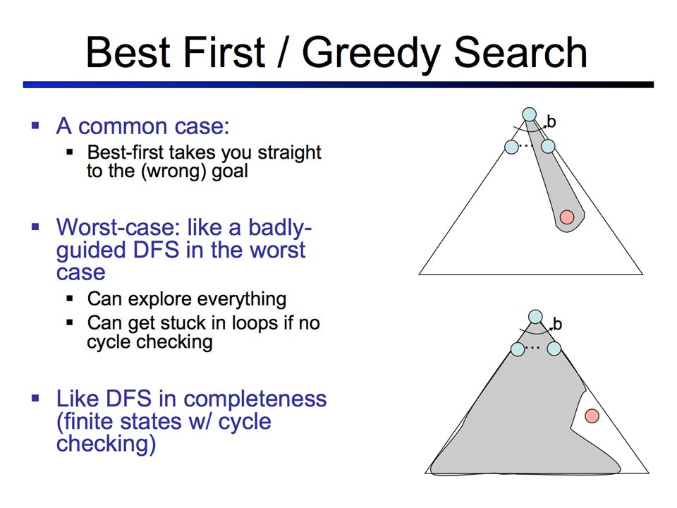
Complete? No – can get stuck in loops start goal So is greedy best-first search complete? No, it can get stuck in infinite loops. Let’s say our start state was iasi and we were trying to get to fageras. Then neamt will be expanded first because it is closest to fagaras. The solution is to go first to vaslui – a step that is actually farther from the goal according to the heuristic – but the algorithm will never find this solution because expanding neamt puts iasi back into the frontier. Iasi is closer to fagaras than vaslui, so iasi will be expanded again, leading to an infinite loop. If we avoid repeated states then GBFS is complete in finite spaces, but not infinite ones.

Complete? No – can get stuck in loops Optimal? No How about optimality? No. in our example the path found sibiu->fagaras->bucharest is 32 kilometers longer than the path through sibiu->RV->pitesti. this is because the algorithm is greedy – at each step it tries to get as close to the goal as it can.

Complete? No – can get stuck in loops Optimal? No Time? Worst case: O(bm) Can be much better with a good heuristic Space? Worst case time and space complexity is O(b^m) where m is the maximum depth of the search space but with a good heuristic function the complexity can be reduced substantially. The amount of reduction depends on the particular problem and on the quality of the heuristic.

How can we fix the greedy problem?
So how can we fix the greedy problem? The greedy solution here will keep greedily choosing the h=1 nodes because they have estimated heuristic smaller than the h=2 node, but this isn’t ideal solution because it’s making lots of steps in the path to the goal.

A* search Idea: avoid expanding paths that are already expensive
The evaluation function f(n) is the estimated total cost of the path through node n to the goal: f(n) = g(n) + h(n) g(n): cost so far to reach n (path cost) h(n): estimated cost from n to goal (heuristic) A* search which dates back to 1968 tries to avoid expanding paths that are already expensive. Here the evaluation function f(n) is the estimated total cost of the path through node n to the goal: f(n) = g(n)+h(n) where g(n) is the true cost so far to reach n (the path cost) and h(n) is the heuristic estimate cost from n to the goal.

A* search example Here’s our romania example with heuristic = straight line distance from node to goal. We start in arad.

A* search example Then the cost of each node on the frontier is the path cost so far + estimate heuristic to get to the goal. Sibiu has lowest f value so we expand it first.

A* search example RV has next lowest f value.

A* search example Now fagaras has lowest f

A* search example Then pitesti

A* search example And we’ve reached bucharest.

Another example Source: Wikipedia
A* with straight line distance heuristic Source: Wikipedia

Uniform cost search vs. A* search
As a side by side comparison UC vs A*. The number of nodes expanded in UCS is significantly higher when compared with the same search problem solved using A* search algorithm Source: Wikipedia

Admissible heuristics
An admissible heuristic never overestimates the cost to reach the goal, i.e., it is optimistic A heuristic h(n) is admissible if for every node n, h(n) ≤ h*(n), where h*(n) is the true cost to reach the goal state from n Is straight line distance admissible? Yes, straight line distance never overestimates the actual road distance When designing a heuristic we consider it’s admissability. An admissible heuristic never overestimates the cost to reach the goal, ie it is always optimistic. Concretely a heuristic h(n) is admissible if for every node n, h(n)<=h*(n) where h*(n) is the true cost to reach the goal state from n. Is straight line distance admissible? Yes because straight line distance never overestimates the actual road distance (b/c the straight line is always the shortest path between two points. Hence it cannot be an overestimate).

Optimality of A* Theorem: If h(n) is admissible, A* is optimal
Proof by contradiction: Suppose A* terminates at goal state n with f(n) = g(n) = C but there exists another goal state n’ with g(n’) < C Then there must exist a node n” on the frontier that is on the optimal path to n’ Because h is admissible, we must have f(n”) ≤ g(n’) But then, f(n”) < C, so n” should have been expanded first! Theorem: if h(n) is admissible then the tree-search A* algorithm is optimal. Let’s use proof by contradiction. Suppose A* terminates at goal state n with f(n)=g(n)=C (f(n)=g(n)+h(n) but since n is a goal state h(n)=0 because it can’t overestimate) but there exists another goal state n’ with g(n’)<C. Then there must exist a node n’’ on the frontier that is on the optimal path to n’ Because h is admissible we must have f(n’’)<=g(n’) But then f(n’’)<C so n’’ should have been expanded first!

Optimality of A* A* is optimally efficient – no other tree-based algorithm that uses the same heuristic can expand fewer nodes and still be guaranteed to find the optimal solution Any algorithm that does not expand all nodes with f(n) ≤ C* risks missing the optimal solution

Properties of A* Complete?
Yes – unless there are infinitely many nodes with f(n) ≤ C* Optimal? Yes Time? Number of nodes for which f(n) ≤ C* (exponential) Space? Exponential

Designing heuristic functions
Heuristics for the 8-puzzle h1(n) = number of misplaced tiles h2(n) = total Manhattan distance (number of squares from desired location of each tile) h1(start) = 8 h2(start) = = 18 Are h1 and h2 admissible? So let’s look at a few example heuristics for the 8-puzzle. We could use a heuristic h1(n)=number of misplaced tiles or h2(n)=total manhattan distance (number of squares from the desired location of each tile). So h1(start)=8 because all tiles are misplaced. H2(start)=3+1+2+…=18 (sum of manhattan distances of each tile to it’s correct placement so tile 7 is 2 down and 1 right=3 from it’s goal location. Tile 2 is 1 right from it’s goal, tile 4 is 1 down and 1 left = 2 from it’s goal…). Are h1 and h2 admissible? H1 = clearly admissible because any out of place tile must be moved at least once. H2 = admissible b/c all any move can do is move one tile one step closer to the goal.

Dominance If h1 and h2 are both admissible heuristics and h2(n) ≥ h1(n) for all n, (both admissible) then h2 dominates h1 Which one is better for search? A* search expands every node with f(n) < C* or h(n) < C* – g(n) Therefore, A* search with h1 will expand more nodes Is either heuristic better than the other? Well if h1 and h2 are both admissible and h2(n)>=h1(n) for all n, then we say that h2 dominates h1. Which one is better for search? A* search expands every node with f(n)<C* ie h(n)<C*-g(n). Therefore, A* search with h1 will expand more nodes. Aka h2 is a better heuristic than h1 because it expands fewer nodes.

Dominance Typical search costs for the 8-puzzle (average number of nodes expanded for different solution depths): d=12 IDS = 3,644,035 nodes A*(h1) = 227 nodes A*(h2) = 73 nodes d=24 IDS ≈ 54,000,000,000 nodes A*(h1) = 39,135 nodes A*(h2) = 1,641 nodes In our 8-puzzle example typical search costs are shown here. For solution depth 12, A* with h1 typically expands 227 nodes and h2 73. for d=24 h1 expands 39k nodes while h2 only expands on average 1600 nodes. So the heuristic does matter although for comparison both of these are heaps better than iterative deepening search which expands 3 million nodes on average for d=12 and 54 billion nodes for d=24.

Heuristics from relaxed problems
A problem with fewer restrictions on the actions is called a relaxed problem The cost of an optimal solution to a relaxed problem is an admissible heuristic for the original problem If the rules of the 8-puzzle are relaxed so that a tile can move anywhere, then h1(n) gives the shortest solution If the rules are relaxed so that a tile can move to any adjacent square, then h2(n) gives the shortest solution Can a computer invent admissible heuristics automatically? One way to get a heuristic is from a relaxed/simplified version of the problem. This is a problem with fewer restrictions on the actions that can be taken. The cost of an optimal solution to a relaxed problem is an admissible heuristic for the original problem. For example, if the rules of the 8-puzzle were changed so that a tile could move anywhere instead of just to an adjacent empty square then h1 would give the exact # of steps to a solution. If the rules were relaxed so that a tile could move to any adjacent square (even to an occupied square), then h2 would give exact # of steps to a solution.

Heuristics from subproblems
Let h3(n) be the cost of getting a subset of tiles (say, 1,2,3,4) into their correct positions Can precompute and save the exact solution cost for every possible subproblem instance – pattern database Another way to get good heuristics is from sub-problems or pattern databases. Here we pre-compute and store solutions to subproblems and then look up their costs as our heuristics. For example in the 8-puzzle, we can precompute the cost of getting a subset of tiles (say 1,2,3,4) into their correct positions without worrying about what happens to the other tiles. This is a lower bound on the cost of the complete problem and turns out to be more accurate than manhattan distance in some cases.

h(n) = max{h1(n), h2(n), …, hm(n)}
Combining heuristics Suppose we have a collection of admissible heuristics h1(n), h2(n), …, hm(n), but none of them dominates the others How can we combine them? h(n) = max{h1(n), h2(n), …, hm(n)} What if we have a collection of admissible heuristics, but none dominates the others for all n. how can we combine them? Well we can just take the max for each n, h(n) = max(h1(n),h2(n),…hm(n)).

Weighted A* search Idea: speed up search at the expense of optimality
Take an admissible heuristic, “inflate” it by a multiple α > 1, and then perform A* search as usual Fewer nodes tend to get expanded, but the resulting solution may be suboptimal (its cost will be at most α times the cost of the optimal solution)

Example of weighted A* search
Heuristic: 5 * Euclidean distance from goal Source: Wikipedia

Example of weighted A* search
Heuristic: 5 * Euclidean distance from goal Source: Wikipedia Compare: Exact A*

Additional pointers Interactive path finding demo
Variants of A* for path finding on grids

All search strategies Algorithm Complete? Optimal? Time complexity
Space complexity BFS DFS IDS UCS Greedy A* If all step costs are equal Yes O(bd) O(bd) No No O(bm) O(bm) If all step costs are equal Yes O(bd) O(bd) Yes Yes Number of nodes with g(n) ≤ C* Worst case: O(bm) No No Best case: O(bd) Yes (if heuristic is admissible) Yes Number of nodes with g(n)+h(n) ≤ C*

Tamara Berg CS Artificial Intelligence

Similar presentations

Presentation on theme: "Tamara Berg CS Artificial Intelligence"— Presentation transcript:

Similar presentations

About project

Feedback

Log in

Auth with social network:

Tamara Berg CS Artificial Intelligence

Similar presentations

Presentation on theme: "Tamara Berg CS Artificial Intelligence"— Presentation transcript:

Similar presentations

About project

Feedback