1. Blind Search by Prof. Jean-Claude Latombe
Russell and Norvig: Chapter 3, Sections 3.4 – 3.6
Slides adapted from:
robotics.stanford.edu/~latombe/cs121/2003/home.htm
by Prof. Jean-Claude Latombe

2. Blind Search Depth first search Breadth first search
Iterative deepening
No matter where the goal is, these algorithms will do the same thing.

3. Depth-First 1
fringe

4. Depth-First 1 2
fringe

5. Depth-First 1 2 3
fringe

6. Breadth First 1
fringe

7. Breadth First 1 2
fringe

8. Breadth First 1 3 2
fringe

9. Breadth First 1 3 2 4
fringe

10. Generic Search Algorithm
Path search(start, operators, is_goal) {
fringe = makeList(start);
while (state=fringe.popFirst()) {
if (is_goal(state))
return pathTo(state);
S = successors(state, operators);
fringe = insert(S, fringe); }
return NULL;
Depth-first: insert=prepend; Breadth-first: insert=append

11. Performance Measures of Search Algorithms
Completeness Is the algorithm guaranteed to find a solution when there is one?
Optimality Is this solution optimal?
Time complexity How long does it take?
Space complexity How much memory does it require?

12. Important Parameters
Maximum number of successors of any state  branching factor b of the search tree
Minimal length of a path in the state space between the initial and a goal state  depth d of the shallowest goal node in the search tree

13. Evaluation of Breadth-first Search
b: branching factor
d: depth of shallowest goal node
Complete
Optimal if step cost is 1
Number of nodes generated: 1 + b + b2 + … + bd = (bd+1-1)/(b-1) = O(bd)
Time and space complexity is O(bd)

14. Big O Notation
g(n) is in O(f(n)) if there exist two positive constants a and N such that:
for all n > N, g(n)  af(n)

15. Time and Memory Requirements
#Nodes
Time
Memory 2
111
.01 msec
11 Kbytes 4
11,111
1 msec
1 Mbyte 6
~106
1 sec
100 Mb 8
~108
100 sec
10 Gbytes 10
~1010
2.8 hours
1 Tbyte 12
~1012
11.6 days
100 Tbytes 14
~1014
3.2 years
10,000 Tb
Assumptions: b = 10; 1,000,000 nodes/sec; 100bytes/node

16. Evaluation of Depth-first Search
b: branching factor
d: depth of shallowest goal node
m: maximal depth of a leaf node
Complete only for finite search tree
Not optimal
Number of nodes generated: 1 + b + b2 + … + bm = O(bm)
Time complexity is O(bm)
Space complexity is O(bm) or O(m)

17. Depth-Limited Strategy
Depth-first with depth cutoff k (maximal depth below which nodes are not expanded)
Three possible outcomes:
Solution
Failure (no solution)
Cutoff (no solution within cutoff)

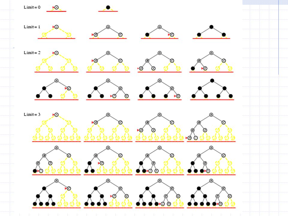
19. Iterative Deepening Strategy
Repeat for k = 0, 1, 2, …:
Perform depth-first with depth cutoff k
Complete
Optimal if step cost =1
Space complexity is: O(bd) or O(d)
Time complexity is: (d+1)(1) + db + (d-1)b2 + … + (1) bd = O(bd)
Same as BFS! WHY???

20. Calculation db + (d-1)b2 + … + (1) bd = bd + 2bd-1 + 3bd-2 +… + db
 bd(Si=1,…, ib(1-i))
= bd (b/(b-1))2

21. Comparison of Strategies
Breadth-first is complete and optimal, but has high space complexity
Bad when branching factor is high
Depth-first is space efficient, but neither complete nor optimal
Bad when search depth is infinite
Iterative deepening is asymptotically optimal

22. Uniform-Cost Strategy
Each step has some cost   > 0.
The cost of the path to each fringe node N is
g(N) =  costs of all steps.
The goal is to generate a solution path of minimal cost.
The queue FRINGE is sorted in increasing cost. S S G A B C 5 1 15 10 1 A 5 B 15 C G 11 G 10

23. Repeated States No Few Many 1 2 3 4 5 6 7 8 search tree is finite
8-queens No
assembly planning
Few 1 2 3 4 5 6 7 8
8-puzzle and robot navigation
Many
search tree is finite
search tree is infinite

24. Avoiding Repeated States
Requires comparing state descriptions
Breadth-first strategy:
Keep track of all generated states
If the state of a new node already exists, then discard the node

25. Avoiding Repeated States
Depth-first strategy:
Solution 1:
Keep track of all states associated with nodes in current path
If the state of a new node already exists, then discard the node
 Avoids loops
Solution 2:
Keep track of all states generated so far
If the state of a new node has already been generated, then discard the node
 Space complexity of breadth-first

26. Summary Search strategies: breadth-first, depth-first, and variants
Evaluation of strategies: completeness, optimality, time and space complexity
Avoiding repeated states