Derek Kern, Roqyah Alalqam, Ahmed Mehzer, Mohammed Mohammed Finding the Limits of Hardware Optimization through Software De-optimization Presented By:

 Flashback  Project Structure  Judging de-optimizations  What does a de-op look like?  General Areas of Focus  Instruction Fetching and Decoding  Instruction Scheduling  Instruction Type Usage (e.g. Integer vs. FP)  Branch Prediction  Idiosyncrasies

 Our Methods  Measuring clock cycles  Eliminating noise  Something about the de-ops that didn’t work  Lots and lots of de-ops

During the research project  We studied de-optimizations  We studied the Opteron For the implementation project  We have chosen de-optimizations to implement  We have chosen algorithms that may best reflect our de- optimizations  We have implemented the de-optimizations  …And, we’re here to report the results

Judging de-optimizations (de-ops)  Whether the de-op affects scheduling, caching, branching, etc, its impact will be felt in the clocks needed to execute an algorithm.  So, our metric of choice will be CPU clock cycles What does a de-op look like?  A de-op is a change to an optimal implementation of an algorithm that increases the clock cycles needed to execute the algorithm and that demonstrates some interesting fact about the CPU in question

 The CPUs  AMD Opteron (Hydra)  Intel Nehalem (Derek’s Laptop)  Our primary focus was the Opteron  The de-optimizations were designed to affect the Opteron  We also tested them on the Intel in order to give you an idea of how universal a de-optimization is  When we know why something does or doesn’t affect the Intel, we will try to let you know

 The code  Most of the de-optimizations are written in C (GCC)  Some of them have a wrapper that is written in C, while the code being de-optimized is written in NASM (assembly)  E.g.  Mod_ten_counter  Factorial_over_array  Typically, if a de-op is written in NASM, then the C wrapper does all of the grunt work prior to calling the de-optimized NASM module

 Problem: How do we measure clock cycles?  An obvious answer  CodeAnalyst  Actually, we were getting strange results from CodeAnalyst  …And, it is hard to separate important code sections from unimportant code sections  …And, it is cumbersome to work with

 A better answer  Embed code that measures clock cycles for important sections  Ok….but how? #if defined(__i386__) static __inline__ unsigned long long rdtsc(void) { unsigned long long int x; __asm__ volatile (".byte 0x0f, 0x31" : "=A" (x)); return x; } #elif defined(__x86_64__) static __inline__ unsigned long long rdtsc(void) { unsigned hi, lo; __asm__ __volatile__ ("rdtsc" : "=a"(lo), "=d"(hi)); return ( (unsigned long long)lo)|( ((unsigned long long)hi)<<32 ); } #endif Answer: Read the CPU Timestamp Counter

 CPU Timestamp Counter  In all x86 CPUs since the Pentium  Counts the number of clock cycles since the last reset  It’s a little tricky in multi-core environments  Care must be taken to control the cores that do the relevant processing

 CPU Timestamp Counter Windows: Linux (Hydra): start /realtime /affinity 4 /b bpsh 11 taskset 0x000000008 Runs the executable on core 3 (of 1 – 4) Runs the executable on node 11, CPU 3 (of 0 – 11) So, by restricting our runs to specific CPUs, we can rely on the CPU timestamp values

 CPU Timestamp Counter  Wrapping code so that clock cycles can be counted // // Send the array off to be counted by the assembly code // unsigned long long start = rdtsc(); #ifdef _WIN64 mod_ten_counter( counts, mod_ten_array, size_of_array ); #elif _WIN32 mod_ten_counter( counts, mod_ten_array, size_of_array ); #elif __linux__ _mod_ten_counter( counts, mod_ten_array, size_of_array ); #endif printf( "Cycles=%d\n", ( rdtsc() - start ) ); The important section is wrapped and the number of clock cycles will be the difference between the start and the finish

 Eliminating noisy results  Even with our precautions, there can be some noise in the clock cycles  So, we need lots of iterations that we can use to generate a good average  But, this can be very, very time consuming  How, oh how? Answer: The Version Tester

 Eliminating noisy results – The Version Tester  Used to iteratively test executables  Expects each executable to return the number of cycles that need to be counted  Remember this? // // Send the array off to be counted by the assembly code // unsigned long long start = rdtsc(); #ifdef _WIN64 mod_ten_counter( counts, mod_ten_array, size_of_array ); #elif _WIN32 mod_ten_counter( counts, mod_ten_array, size_of_array ); #elif __linux__ _mod_ten_counter( counts, mod_ten_array, size_of_array ); #endif printf( "Cycles=%d\n", ( rdtsc() - start ) );

 Eliminating noisy results – The Version Tester  Runs executables for specified number of iterations and then averages the number of cycles > bpsh 10 taskset 0x000000004 version_tester mtc.hydra-core3.config Running Optimized for 1000 for 200 iterations Done running Optimized for 1000 with an average of 19058 cycles Running De-optimized #1 for 1000 for 200 iterations Done running De-optimized #1 for 1000 with an average of 21039 cycles Running Optimized for 10000 for 200 iterations Done running Optimized for 10000 with an average of 187296 cycles Running De-optimized #1 for 10000 for 200 iterations Done running De-optimized #1 for 10000 with an average of 206060 cycles Example run on Hydra: Runs version_tester.exe on CPU 2 and mod_ten_counter.exe on CPU 3

 Eliminating noisy results – The Version Tester  Running version_tester Command Format Configuration File (for Hydra) ITERATIONS=200 __EXECUTABLES__ Optimized for 1000=taskset 0x000000008./mod_ten_counter_op 1000 De-optimized #1 for 1000=taskset 0x000000008./mod_ten_counter_deop 1000 Optimized for 10000=taskset 0x000000008./mod_ten_counter_op 10000 De-optimized #1 for 10000=taskset 0x000000008./mod_ten_counter_deop 10000 Optimized for 100000=taskset 0x000000008./mod_ten_counter_op 100000 De-optimized #1 for 100000=taskset 0x000000008./mod_ten_counter_deop 100000 Optimized for 1000000=taskset 0x000000008./mod_ten_counter_op 1000000 De-optimized #1 for 1000000=taskset 0x000000008./mod_ten_counter_deop 1000000

 Eliminating noisy results – The Version Tester  Running Configuration File (for Windows): ITERATIONS=200 __EXECUTABLES__ Optimized for 10=.\mod_ten_counter\mod_ten_counter_op 10 De-optimized #1 for 10=.\mod_ten_counter\mod_ten_counter_deop 10 Optimized for 100=.\mod_ten_counter\mod_ten_counter_op 100 De-optimized #1 for 100=.\mod_ten_counter\mod_ten_counter_deop 100 Optimized for 1000=.\mod_ten_counter\mod_ten_counter_op 1000 De-optimized #1 for 1000=.\mod_ten_counter\mod_ten_counter_deop 1000 Optimized for 10000=.\mod_ten_counter\mod_ten_counter_op 10000 De-optimized #1 for 10000=.\mod_ten_counter\mod_ten_counter_deop 10000 Optimized for 100000=.\mod_ten_counter\mod_ten_counter_op 100000 De-optimized #1 for 100000=.\mod_ten_counter\mod_ten_counter_deop 100000 Optimized for 1000000=.\mod_ten_counter\mod_ten_counter_op 1000000 De-optimized #1 for 1000000=.\mod_ten_counter\mod_ten_counter_deop 1000000 Optimized for 10000000=.\mod_ten_counter\mod_ten_counter_op 10000000 De-optimized #1 for 10000000=.\mod_ten_counter\mod_ten_counter_deop 10000000

 Eliminating noisy results – The Version Tester  Therefore, using the Version Tester, we can iterate hundreds or thousands of times in order to obtain a solid average number cycles  So, we believe our results fairly represent the CPUs in question

 You are going to see the various de-optimizations that we implemented and the corresponding results  These de-optimizations were tested using the Version Tester and were executed while restricting the execution to a single core (CPU)

 …something about the de-optimizations that were less than successful  Branch Patterns  Remember: We wanted to challenge the CPU with branching patterns that could force misses  This turned out to be very difficult to do  Random data caused a significant slowdown. But random data will break any branch prediction mechanism  The branch prediction mechanism on the Opteron is very very good

 Unpredictable Instructions - Recursion  Remember: Writing recursive functions that call other functions near their return  This was supposed to overload the return address buffer and cause mispredictions  It turned out to be very difficult to implement  We never really showed any performance degradation  So, don’t worry about this one

So, without further adieu...

De-Optimization Results Area: Instruction Scheduling Dependency Chain

 Description  As we have seen in this class data dependency would have an impact on the ILP.  Dynamic scheduling as we saw can eliminate the WAW & WAR dependency  However, to a point the Dynamic scheduling could be overwhelmed which could affect the performance as we will see next  The Opteron  Opetron,like all the other architectures, would be highly affected by the data hazard  The reason of this de-optimization is to show the impact of the data chain dependency on the performance

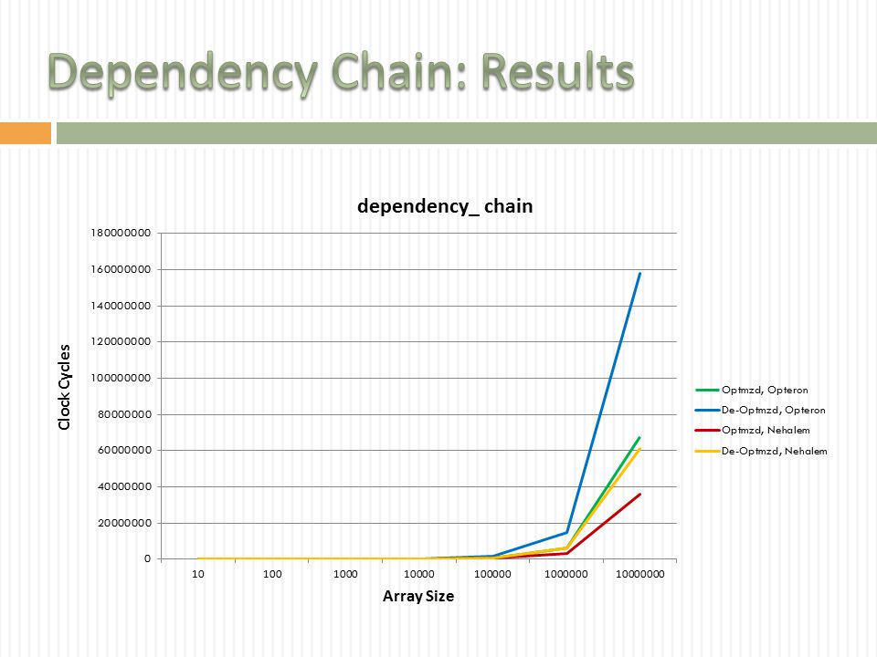
 dependency_chain.exe  We implemented two versions of a program called ‘dependency_chain’  The program takes an array size as argument  It then generates an array of the specified size in which each element is populated with integers x where 0 <= x <= 20  The array’s element are being summed and the output would be the number of cycles that been taken by the program

 dependency_chain.exe  In the optimized version adds the elements of the array by striding through the array in four element chunks and adding elements to four different temporary variables  Then the four temporary variables are added  The advantage is allowing four large dependency chain instead of one massive one  However for the de-optimized version, each of the element of the array are sums into one variable  This create a massive dependency chain which will quickly exhausts the scheduling resources of the dynamic scheduler

 Dependency_chain.exe for ( i = 0; i < size_of_array; i+=4 ) { sum1 += test_array[i]; sum2 += test_array[i + 1]; sum3 += test_array[i + 2]; sum4 += test_array[i + 3]; } sum = sum1 + sum2 + sum3 + sum4; for ( i = 0; i < size_of_array; i++ ) { sum += test_array[i]; } Optimized De-Optimized Source

 dependency_chain.exe  chart below shows that not breaking up a dependency chain can be extraordinarily costly. On the Opteron, it caused ~150% for all array sizes.  The scheduling resources of the Opteron become overwhelmed essentially causing the program to run sequentially, i.e. with no ILP  Nehalem was impacted by this de-optimization too. Given the lesser impact, one can only imagine that it has more scheduling resources Difference between Optimized and De-Optimized Versions Array SizeAMD Opteron: Difference Slowdown(%)Intel Nehalem: Difference Slowdown(%) 10807.07212.58 10015100.88243632.15 10001042911.61-990-1.24 1000011597512.76361585.33 100000113974812.592388523.54 10000001152962412.66-3505949-5.42 1000000017519177418.9030815570.51 * In Clock Cycles Array SizeAMD Opteron: Difference Slowdown(%)Intel Nehalem: Difference Slowdown(%) 10 43 19.03 3 2.5 100 841 120.31 256 57.66 1000 8857 160.02 2793 79.03 10000 87503 160.64 30073 86.46 100000 877172 155.3 272096 78.83 1000000 8633066 142.06 2937193 88.53 10000000 90226731 132.98 25436239 71.12

 Lessons  The code for the de-optimization is so natural that it is a little scary. It is elegant and parsimonious  However, this elegance and parsimony may come at a very high cost  If you don’t get the performance that you expect from a program, then it is definitely worth looking for these types of dependency chains  Break these chains up to give dynamic schedulers more scheduling options

High Instructions Latency De-Optimization Results Area: Instruction Fetching and Decoding

 Description  CPUs often have instructions that can perform almost the same operation  Yet, in spite of their seeming similarity, they have very different latencies. By choosing the high-latency version when the low latency version would suffice, code can be de-optimized  The Opetron  The LOOP instruction on the Opteron has a latency of 8 cycles, while a test (like DEC) and jump (like JNZ) has a latency of less than 4 cycles  Therefore, substituting LOOP instructions for DEC/JNZ combinations will be a de-optimization

 fib.exe  We implemented a program called ‘fib’  It takes an array size as an argument  Fibonacci number is calculated for each element in the array

 fib.exe  Fibonacci number is calculated in assembly code  In the optimized version used dec & jnz instructions which take up to 4 cycles  In the de-optimized version used loop instruction which takes 8 cycles

 fib.exe calculate: mov edx, eax add ebx, edx mov eax, ebx mov dword [edi], ebx add edi, 4 dec ecx jnz calculate calculate: mov edx, eax add ebx, edx mov eax, ebx mov dword [edi], ebx add edi, 4 loop calculate Optimized De-Optimized Source

 fib.exe 08048481 : 8048481: 89 c2 mov %eax,%edx 8048483: 01 d3 add %edx,%ebx 8048485: 89 d8 mov %ebx,%eax 8048487: 89 1f mov %ebx,(%edi) 8048489: 81 c7 04 00 00 00 add $0x4,%edi 804848f: 49 dec %ecx 8048490: 75 ef jne 8048481 08048481 : 8048481: 89 c2 mov %eax,%edx 8048483: 01 d3 add %edx,%ebx 8048485: 89 d8 mov %ebx,%eax 8048487: 89 1f mov %ebx,(%edi) 8048489: 81 c7 04 00 00 00 add $0x4,%edi 804848f: e2 f0 loop 8048481 Optimized De-Optimized Compiled

 fib.exe  In the chart below we can see that optimized version significantly outperforms the de-optimized version. The results on Nehalem are more impressive Difference between Optimized and De-Optimized Versions Array SizeAMD Opteron: Difference Slowdown(%)Intel Nehalem: Difference Slowdown(%) 10807.07212.58 10015100.88243632.15 10001042911.61-990-1.24 1000011597512.76361585.33 100000113974812.592388523.54 10000001152962412.66-3505949-5.42 1000000017519177418.9030815570.51 * In Clock Cycles Array SizeAMD Opteron: Difference Slowdown(%)Intel Nehalem: Difference Slowdown(%) 10 17 9.04 9 8.57 100 155 29.4 244 81.87 1000 1386 34.74 2239 104.52 10000 14588 22.03 19519 62.16 100000 123271 17.91 256839 87.42 1000000 1206678 16.94 2430301 81.51 10000000 11716747 14.07 19896396 65.26

 Lessons  As we have seen different instructions can affect your program when you don’t choose them carefully.  It’s important to know which instruction takes more cycles to avoid using them as possible.

Costly Instructions De-Optimization Results Area: Instruction Type Usage

 Description  Some instructions can do the same job but with more cost in term of number of cycles  The Opetron  Integer division for Opetron costs 22-47 cycles for signed, and 17-41 unsigned  While it takes only 3-8 cycles for both signed and unsigned multiplication

 mult_vs_div_deop_1.exe & mult_vs_div_op.exe  We implemented two programs, optimized and de-optimized versions  They take an array size as an argument, the array initialized randomly with powers of 2 (less than or equal to 2^12)  The de-optimized version divides each element by 2.0. The optimized version multiplies each element by 0.5.  The versions are functionality equivalent

 mult_vs_div_deop_1.exe & mult_vs_div_op.exe for ( i = 0; i < size_of_array; i++ ) { test_array[i] = test_array[i] / 2.0; } for ( i = 0; i < size_of_array; i++ ) { test_array[i] = test_array[i] * 0.5; } De-optimized Optimized

 mult_vs_div_deop_1.exe & mult_vs_div_op.exe  By looking to the chart below you can see this de-optimization has a huge impact on the Opetron of average 23%. It still has an affect on the Nehalem even it is not as big as the Opetron Difference between Optimized and De-Optimized Versions * In Clock Cycles Array SizeAMD Opteron: Difference Slowdown(%)Intel Nehalem: Difference Slowdown(%) 10 99 18.1 -42 -14.34 100 949 24.73 57 2.04 1000 9754 26.49 1630 5.96 10000 94658 25.67 16364 5.07 100000 938712 25.27 117817 4.54 1000000 9619257 23.94 675940 2.64 10000000 96477334 23.98 8585454 3.41

 Lessons  Small changes in your code could have a real impact on the performance  It so important to know the difference between instruction in term of cost  Seek discount instruction when it is possible

De-Optimization Results Area: Instruction Type Usage Costly Instructions

 Description  Some instructions can do the same job but with more cost in term of number of cycles Example: float f1, f2 if (f1<f2) This is a common usage for programmer which could be considered a de- optimization technique  The Opteron  Branches based on floating-point comparisons are often slow

 Compare_two_floats.exe  We implemented a program called ‘Compare_two_floats’  It takes a number of iteration as an argument  Comparisons between 2 floating numbers will be done in this program.

 Compare_two_floats_deop.exe & Compare_two_floats_op.exe  In the de-optimized version we compare two floats by using the old common way as we will see in the next slide  However for the optimized version, we used change the float to integer and take it as a condition instead  The condition was specified on purpose to be not taken all the time

 Compare_two_floats_deop.exe & Compare_two_floats_op.exe Optimized De-Optimized for (i = 0; i <numberof_iteration ; i++) { if (f1<=f2) { Count_numbers(i); count++; } else count++; } for (j = 0; j <numberof_iteration ; j++) { if (FLOAT2INTCAST(t)<=0) { Count_numbers(i); count++; } else count++; }

 Compare_two_floats.exe

 The chart below shows a small impact on the Opetron, however the results were surprising for the Nehalem even it was designated basically for the Opetron. Difference between Optimized and De-Optimized Versions Array SizeAMD Opteron: Difference Slowdown(%)Intel Nehalem: Difference Slowdown(%) 10 -10991 -97.19 43 26.70 100 -10960 -86.18 471 49.68 1000 -9892 -37.97 5285 59.90 10000 -982 -0.60 52211 58.82 100000 88962 5.86 413932 41.79 1000000 987559 6.56 4298502 44.46 10000000 9949917 6.62 41906333 46.14 * In Clock Cycles

 Lessons  Usually floats comparison are more expensive compare to integer in term of number of cycles  Even though the Opetron passed this test, that does not mean your computer will do the same!!  The float comparisons still have a big impact on the Nehalem  Again, great care must be taken when the program deals with more floats comparison.

De-Optimization Results Area: Instruction Scheduling Loop Re-rolling

 Description  Loops not only affect branch prediction. They can also affect dynamic scheduling. How ?  Having two instructions 1 and 2 be within loops A and B, respectively. 1 and 2 could be part of a unified loop. If they were, then they could be scheduled together. Yet, they are separate and cannot be  The Opteron  Given that the Opteron is 3-way scalar, this de-optimization could significantly reduce IPC  This would be two consecutive loops each containing one or more instructions such that the loops could be combined

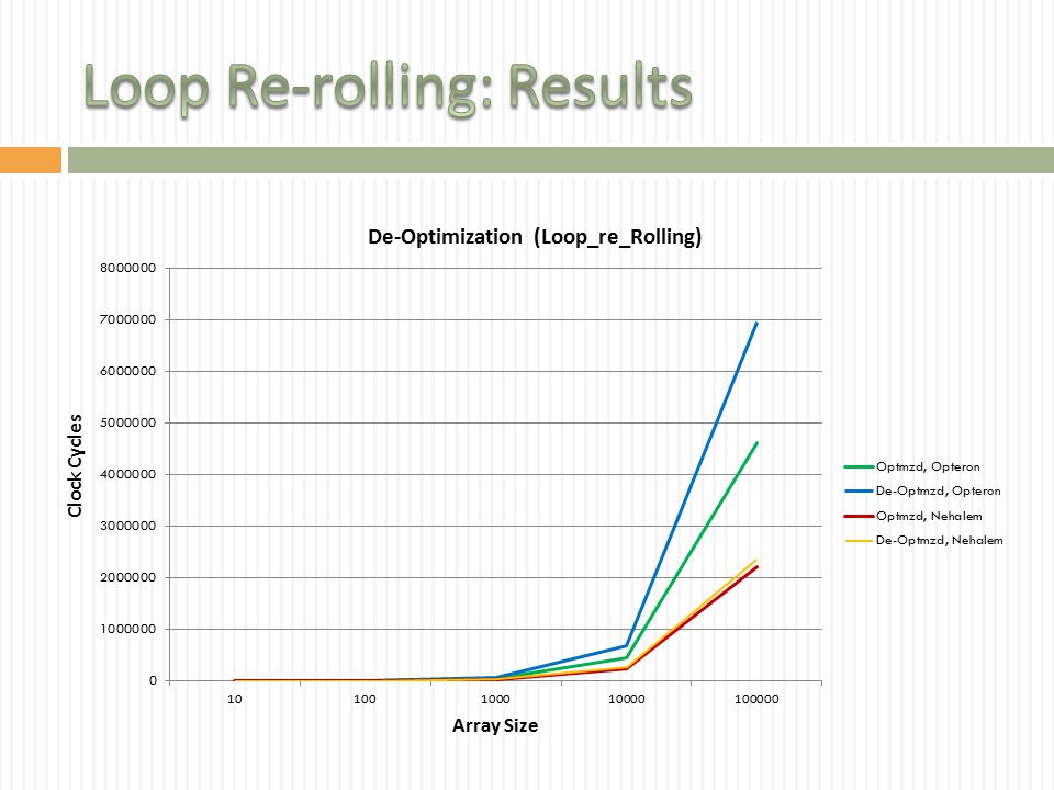
 Loop_re_rolling_deop.exe & loop_re_rolling_op.exe  We implemented two programs : optimized and de-optimized versions  They take an array size as an argument, and initialize it randomly  Cubic and quadratic are calculated for each element in the array  In the de-optimized version the cubic and quadratic calculation were in two consecutive loops. They are combined with the same loop for the optimized version.  Bothe versions are functionality equivalent

 Loop_re_rolling_deop.exe & loop_re_rolling_op.exe  We want to show whether the removing some of the flexibility available to the dynamic scheduler would affect the number of cycles or not.  It is not expected for the de-optimization instructions to be scheduled at the same time. The de-optimization should prevent this

 Loop_re_rolling_deop.exe & loop_re_rolling_op.exe Optimized De-optimized for (i=0;i<size_of_array;i++) { quadratic_array[i]=load_store_array[i]*load_store_array[i]; } for (i=0;i<size_of_array;i++) { cubic_array[i]=load_store_array[i]*load_store_array[i]*load_store_array[i]; } for (i=0;i<size_of_array;i++) { quadratic_array[i]=load_store_array[i]*load_store_array[i]; cubic_array[i]=load_store_array[i]*load_store_array[i]*load_store_array[i]; }

 Loop_re_rolling_deop.exe & loop_re_rolling_op.exe  The slow percentage is defiantly large for Opetron. It is almost 50% in average.  It is large for the Nehalem as well.  These results shows the difference between using dynamic scheduling or not Difference between Optimized and De-Optimized Versions * In Clock Cycles Array SizeAMD Opteron: Difference Slowdown(%)Intel Nehalem: Difference Slowdown(%) 1018943.958328.32 100165353.6835715.35 10002131154.96469621.28 1000023433652.423931117.10 100000235232850.931347866.05

 Lessons  Dynamic scheduling is absolutely important  Loops should be used carefully, and enroll them when it is possible  Instructions that do not depend on each other (No true dependency), would guarantee a better dynamic scheduling that would enhance the performance especially when they are repeated frequently

Store-to-load dependency De-Optimization Results Area: Instruction Type Usage

 Description  Store-to-load dependency takes place when stored data needs to be used shortly  This type of dependency increases the pressure on the load and store unit and might cause the CPU to stall especially when this type of dependency occurs frequently  In many instructions, when we load the data which is stored shortly  The Opteron

 dependecy_deop.exe & dependency_op.exe  We implemented two versions of dependency program, one for optimization and the other for de-optimization  They take an array size as an argument, the array initialized randomly  Both versions perform a prefix sum over the array. Thus, the final array element will contain a sum with it and all previous elements within the array

 dependecy_deop.exe & dependency_op.exe  In the de-optimization we are storing and loading shortly the same elements of the array  However, we used a temporary variables to avoid this type of dependency in the optimized version  The optimization code has more instructions, and it is obvious that adding more instructions would have impact on the number of cycles compare to the version that has fewer instructions

 dependecy_deop.exe & dependency_op.exe Optimized for ( i = 1; i < size_of_array; i++ ) { test_array[i] = test_array[i] + test_array[i - 1]; } for ( i = 3; i < size_of_array; i += 3 ) { temp2 = test_array[i - 2] + temp_prev; temp1 = test_array[i - 1] + temp2; test_array[i - 2] = temp2; test_array[i - 1] = temp1; test_array[i] = temp_prev = test_array[i] + temp1; } De-optimized

 dependecy_deop.exe & dependency_op.exe  The chart below we can see it this de-optimization technique has an average 60% of slowing down for the Opetron, which is a huge difference. The Nehalem as well has been affected by this code Difference between Optimized and De-Optimized Versions * In Clock Cycles Array SizeAMD Opteron: Difference Slowdown(%)Intel Nehalem: Difference Slowdown(%) 10 87 37.5 12 8.16 100 2392 77.98 230 21.9 1000 9858 78.41 1610 15.38 10000 79180 63.89 17517 17.84 100000 786708 63.1 176893 18.7 1000000 8181981 64.12 1205000 12.12 10000000 81498679 58.83 17276216 18.06

 Lessons  Load-store dependency is something you should be aware of  Writing more instructions does not always mean your program will run slower  Avoid this common usage of load store dependency to have a good impact on your program

De-Optimization Results Area: Instruction type usage Costly Behavior

 Description  Conditional statement is an active player in almost everyone’s code. Would you believe if someone tells you a minor change could have a real effect on your program?  The sequence of the statements that are needed to be checked is SO IMPORTANT.  Most of the architectures use the same sequence to check these condition regardless the programming language you use & the platform.

 IF_Condition.exe  We implemented two versions of a program called ‘IF_Condition’  The takes a number of iterations as an argument and initialize an array randomly with floats between 0.5 and 11.0  For each element in the array, we add one to a dummy variable if its index is equal to 0 (mod 2) and its value is greater than 1.5.

 IF_deop.exe & IF_op.exe  The if statement will hold true if both conditions are true  In the de-optimized version we put the condition that has more chance to be false as second condition,while we put it a first one in the optimized version

 IF_deop.exe & IF_op.exe Optimized De-Optimized for ( i = 0; i < size_of_array; i++ ) { mod = ( i % 2 ); if ( test_array[i] > 1.5 && mod == 0 ) dummy++; else dummy--; } for ( i = 0; i < size_of_array; i++ ) { mod = ( i % 2 ); if ( mod == 0 && test_array[i] > 1.5 ) dummy++; else dummy--; }

 IF_Condition.exe  The chart below shows optimized version outperforms the de-optimized version on both the Opetron and Nehalem. Difference between Optimized and De-Optimized Versions Array SizeAMD Opteron: Difference Slowdown(%)Intel Nehalem: Difference Slowdown(%) 10 -207 -26.90 57 23.85 100 338 15.48 990 56.99 1000 6438 38.27 4886 33.86 10000 63975 38.09 47374 37.87 100000 651438 38.94 520198 50.64 1000000 6385986 37.37 4577710 41.86 10000000 66023847 35.89 49997484 47.52 * In Clock Cycles

 Lessons  Conditional statements can have a negative impacts if they are ignored  One case was implemented (&&), and other cases would be equivalent in term of increasing the number of cycles  If it is possible to specify which conditions will be more true or false then putting that condition in the right position will save some cycles

De-Optimization Results Area: Branch Prediction Branch Density

 Description  This de-optimization attempts to overwhelm the CPUs ability to predict a branch code by packing branches as tightly as possible  Whether or not a bubble is created is dependent upon the hardware  However, at some point, the hardware can only predict so much and pre-load so much code  The Opteron  The Opteron's BTB (Branch Target Buffer) can only maintain 3 (used) branch entries per (aligned) 16 bytes of code [AMD05]  Thus, the Opteron cannot successfully maintain predictions for all of the branches within following sequence of instructions

401399: 8b 44 24 10 mov 0x10(%esp),%eax 40139d: 48 dec %eax 40139e: 74 7a je 40141a 4013a0: 8b 0f mov (%edi),%ecx 4013a2: 74 1b je 4013bf 4013a4: 49 dec %ecx 4013a5: 74 1f je 4013c6 4013a7: 49 dec %ecx 4013a8: 74 25 je 4013cf 4013aa: 49 dec %ecx 4013ab: 74 2b je 4013d8 4013ad: 49 dec %ecx 4013ae: 74 31 je 4013e1 4013b0: 49 dec %ecx 4013b1: 74 37 je 4013ea 4013b3: 49 dec %ecx 4013b4: 74 3d je 4013f3 4013b6: 49 dec %ecx 4013b7: 74 43 je 4013fc 4013b9: 49 dec %ecx 4013ba: 74 49 je 401405 4013bc: 49 dec %ecx 4013bd: 74 4f je 40140e

 mod_ten_counter.exe  We implemented a program called ‘mod_ten_counter’  It takes an array size as an argument  The array is populated with a repeating pattern of consecutive integers from zero to nine  Like: 012345678901234567890123456789…  In other words, the contents are not random  Very simply, it counts the number of times that each integer (0 – 9) appears within the array

 mod_ten_counter.exe  The optimized version maintained proper spacing between branch instructions  The de-optimized version (seen on the previous slide) has densely packed branches  Notes:  The spacing for the optimized version is achieved with NOP instructions  It has one extra NOP per branch so it has roughly 5 more instructions per iteration than the de-optimized version  Thus, if the optimized version outperforms the de-optimized version, then the difference will be even more impressive

 mod_ten_counter.exe cmp ecx, 0 je mark_0 ; We have a 0 nop dec ecx je mark_1 ; We have a 1 nop dec ecx je mark_2 ; We have a 2 nop dec ecx je mark_3. cmp ecx, 0 je mark_0 ; We have a 0 dec ecx je mark_1 ; We have a 1 dec ecx je mark_2 ; We have a 2 dec ecx je mark_3. Optimized De-Optimized Source

 mod_ten_counter.exe

 As you can see from the chart below, in spite of its handicap, the optimized version significantly outperforms the de-optimized version  Interestingly, this de-optimization is more impressive on the Intel, even though it was designed with the Opteron in mind Difference between Optimized and De-Optimized Versions * In Clock Cycles Array SizeAMD Opteron: Difference Slowdown(%)Intel Nehalem: Difference Slowdown(%) 10-47-7.31399.92 1001857.8033127.36 1000223411.86635589.42 100002323012.6967653110.38 10000020376010.9853736284.27 100000016206528.40530676689.63 10000000172630488.345208297178.85

 So, what’s up with the Nehalem?  The Nehalem performs well generally, but is very susceptible to this de- optimization. Why?  There isn’t great information on this facet of the Nehalem  But…  The Nehalem can handle 4 active branches per 16 bytes  The misprediction penalty is ~17 cycles so the Nehalem has a long pipeline  Therefore, missing the BTB is probably very costly as well

 Lessons  Branch density can adversely affect performance and make otherwise predictable branches unpredictable  Great care must be taken when designing branches, if-then-else structures and case-switch structures

De-Optimization Results Area: Branch Prediction Unpredictable Instructions

 Description  Some CPUs restricts only one branch instruction be within a certain number bytes  If this exceeded or if branch instructions are not aligned properly, then branches cannot be predic ted  The Opteron  The return (RET) instruction may only take up one byte  If a branch instruction immediately precedes a one byte RET instruction, then RET cannot be predicted  One byte RET instruction can cause a miss prediction even if we have one branch instruction per 16 bytes  Alignment: 9 branch indicators associated with byte addresses of 0,1,3,5,7,9,11, 13, & 15 within each 16 byte segment

 factorial_over_array.exe  We implemented a program called ‘factorial_over_array’  It takes an array size as an argument  The array is populated with random integers between 1 and 12 e.g. { 3, 7, 4, 10, 9, 1, 5, 2, 12 }  Factorial is calculated for each element in the array

 factorial_over_array.exe  Factorial is calculated in assembly code  In the optimized version, the RET instruction is aligned using a NOP so that it is not immediately next another branch and so that it falls on an odd number within the 16 byte segment  In the de-optimized version, the RET instruction is aligned immediately next to a branch instruction and so that it falls on an even number within the 16 byte segment

 factorial_over_array.exe global _factorial section.text _factorial: nop mov eax, [esp+4] cmp eax, 1 jne calculate nop ret calculate: dec eax push eax call _factorial add esp, 4 imul eax, [esp+4] ret global _factorial section.text _factorial: nop mov eax, [esp+4] cmp eax, 1 jne calculate ret calculate: dec eax push eax call _factorial add esp, 4 imul eax, [esp+4] ret Optimized De-Optimized Source

 factorial_over_array.exe 0: 90 nop 1: 8b 44 24 04 mov 0x4(%esp),%eax 5: 83 f8 01 cmp $0x1,%eax 8: 75 02 jne c a: 90 nop b: c3 ret c: 48 dec %eax d: 50 push %eax e: e8 ed ff ff ff call 0 13: 83 c4 04 add $0x4,%esp 16: 0f af 44 24 04 imul 0x4(%esp),%eax 1b: c3 ret 0: 90 nop 1: 8b 44 24 04 mov 0x4(%esp),%eax 5: 83 f8 01 cmp $0x1,%eax 8: 75 01 jne b a: c3 ret b: 48 dec %eax c: 50 push %eax d: e8 ee ff ff ff call 0 12: 83 c4 04 add $0x4,%esp 15: 0f af 44 24 04 imul 0x4(%esp),%eax 1a: c3 ret Optimized De-Optimized Compiled

 factorial_over_array.exe

 As you can see from the chart below, the optimized version significantly outperforms the de-optimized version  Interestingly, this de-optimization has an inconclusive effect on the Nehalem Difference between Optimized and De-Optimized Versions Array SizeAMD Opteron: Difference Slowdown(%)Intel Nehalem: Difference Slowdown(%) 10807.07212.58 10015100.88243632.15 10001042911.61-990-1.24 1000011597512.76361585.33 100000113974812.592388523.54 10000001152962412.66-3505949-5.42 1000000017519177418.9030815570.51 * In Clock Cycles Array SizeAMD Opteron: Difference Slowdown(%)Intel Nehalem: Difference Slowdown(%) 10807.07212.58 10015100.88243632.15 10001042911.61-990-1.24 1000011597512.76361585.33 100000113974812.592388523.54 10000001152962412.66-3505949-5.42 1000000017519177418.9030815570.51

 Lessons  Alignment is one of many ways that instructions can become unpredictable  These constant misses can be very costly  Again, great care must be taken. Brevity, at times, can create inefficiencies

 We’ve shown you lots of de-optimizations  Most of them were successful  So, now, you know some of the costs associated with ignoring CPU architecture when writing code  If you are like us, then you must be reconsidering how you write software  As you’ve seen, some of the simple habits that you’ve accumulated may be causing your code to run more slowly than it would have otherwise

[AMD05] AMD64 Technology. Software Optimization Guide for AMD64 Processors, 2005 [AMD11] AMD64 Technology. AMD64 Architecture Programmers Manual, Volume 1: Application Programming. 2011 [AMD11] AMD64 Technology. AMD64 Architecture Programmers Manual, Volume 2: System Programming. 2011 [AMD11] AMD64 Technology. AMD64 Architecture Programmers Manual, Volume 3: General Purpose and System Instructions. 2011

Derek Kern, Roqyah Alalqam, Ahmed Mehzer, Mohammed Mohammed Finding the Limits of Hardware Optimization through Software De-optimization Presented By:

Similar presentations

Presentation on theme: "Derek Kern, Roqyah Alalqam, Ahmed Mehzer, Mohammed Mohammed Finding the Limits of Hardware Optimization through Software De-optimization Presented By:"— Presentation transcript:

Similar presentations

About project

Feedback

Log in

Auth with social network:

Derek Kern, Roqyah Alalqam, Ahmed Mehzer, Mohammed Mohammed Finding the Limits of Hardware Optimization through Software De-optimization Presented By:

Similar presentations

Presentation on theme: "Derek Kern, Roqyah Alalqam, Ahmed Mehzer, Mohammed Mohammed Finding the Limits of Hardware Optimization through Software De-optimization Presented By:"— Presentation transcript:

Similar presentations

About project

Feedback