1. Electronic Energy Transfer in Molecular Aggregates: Theoretical Approaches from Förster, Redfield and beyond Co-workers: Jianshu Cao, Xin Chen, Eric Zimanyi, Seogjoo Jang,Yuan-Chung Cheng, Alberto Suarez, Irwin Oppenheim Experimental colleagues: G. Scholes (Toronto), J. Kohler (Bayreuth), S. Volker (Leiden)

2. Förster 1948 Formula for Resonance Energy Transfer in terms of donor emission and acceptor absorption (  rad /  D ) = 1 +  rad /  ET = 1 + (R o /R) 6 R o calculated from the overlap of donor emission and acceptor absorption which provides a measurement of R Single donor and large number of random acceptors leads to exponential fluorescence. Today, used as a biological ruler in many single molecule experiments.

5. Recent extensions: multi-chromophoric donors and acceptors; application to light harvesting complexes (Sumi et al; Scholes; Jang, Newton, RJS; Cheng & RJS); Review of the assumptions of model: Beljonne, Curutchet, Scholes, RJS (JPCB 2009)

6. Förster Resonance Energy Transfer H = (1/2)    P D    D   Q D   } + (1/2)    P A    A   Q A   } + [E D +   g D Q D  ] |D e A g > <D g A e | + J { |D e A g > <D e A g | } J = Coulomb interaction between D and A -- in the multipole expansion this becomes a (transition) dipole dipole interaction ~ 1/R 3 Note the close resemblance to the Marcus model for electron transfer. Use 2nd order perturbation theory (Fermi Golden Rule) starting from the eigenstates of H with J=0 (polaron or displaced oscillator states).

7. Davydov: The Theory of Molecular Excitons In 1948, Davydov’s book was published in Russia and translated by Kasha in the 1950’s. Davydov was only interested in coherences: His treatment of the electronic states of molecular crystals was like band theory in solid state physics. The states were superpositions of site (excited) states with translational invariance. Davydov was interested in low temperature spectroscopy of organic solids; Förster was interested in molecular fluorescence in solution.

8. Moderate to Strong Electronic Interactions Between Donor and Acceptor When both coherent and incoherent processes take place, there are many possible theoretical descriptions (which are often rearrangements of others), usually involving the reduced density matrix (that is, the density matrix for the entire system averaged over the thermal environment). Some names are: stochastic Liouville equation (SLE), Generalized Master Equation (GME), Bloch equation, Redfield theory, Lindblad form, Completely Ordered Perturbation (COP), Partially Ordered Perturbation (POP),... In all of these methods, it is difficult to go beyond second order in the perturbation, so one has to be careful in choosing how to form H 0 + V from H.

9. Redfield Model: Coherence, decoherence, and all that H = H 0 + V = H sys + H bath + V d  /dt = -i [H,  ];  (t) = Tr bath   (0) =  (0)  bath equ (assumption) d  (t)/dt = -i [H sys,  (t)] - ∫ 0 t K(  )  (t-  d  Exact! Redfield: bath relaxes much faster than system, so K decays quickly, then d  (t) /dt = -i [H sys,  (t)] - R  (t  R(ij,kl) given in terms of infinite integrals over time correlation functions of matrix elements of V (in the system eigenstates representation). Note well: the Redfield model is a weak coupling model, and depends on how you choose H 0 and V. It has problems if you are not careful.

10. Redfield Model: Coherence, decoherence, and all that Consider a two state system, like the Förster model. H sys has eigenstates |1> and |2> (eigenstates of H sys not site states!), then  11 and  22 are populations and  12 and  21 are coherences. The general Redfield model will have coupling terms between populations and coherences. The secular approximation neglects these and then (A = exp[- (E 1 -E 2 )/T]) d(  11 -  22 )/dt = -(1-A)  - (1+A)  (  11 -  22 ) d  12 /dt = {-i(E 1 -E 2 ) - {  pd +(1+A)  /2}}  12 +(1+A)  /2  21

11. Redfield Model: Coherence, decoherence, and all that  ∫ -∞ ∞ exp[i(E 1 -E 2 )t]dt; = Fermi Golden Rule for transitions from 1 to 2  pd  ∫ -∞ ∞ dt Pure dephasing rate (fluctuation of eigenenergy due to bath) The terms coupling coherences and populations are related to ∫ -∞ ∞ exp(i  t)dt for  = 0 and  = E 1 -E 2

12. Redfield Model: Coherence, decoherence, and all that Let’s naively apply this to the Förster problem : choose H sys = E D |D e A g > <D e A g | } V=   g D Q D  |D e A g > <D g A e | Now the zeroth order states are “exciton” states (linear combinations of the site states) and the perturbation term only allows one quantum jumps in the vibrational modes. Leads to incorrect FRET formula! What went wrong? We chose the wrong zeroth order Hamiltonian. This is a common mistake in thinking about energy transfer, coherence and decoherence.

13. Polaron Transformation To repair this, we must choose a different zeroth order Hamiltonian. One good way to do this is to transform the Hamiltonian by a unitary transformation that diagonalizes the V in the site representation, that is, form polaron site functions. This transforms the electronic coupling term to J exp[   g D P D      g A P A     |D e A g > <D e A g |  H.c. Now average this over the bath density matrix to get = Jexp(-S) and add and subtract this average from the Hamiltonian. Finally,

14. Polaron Transformation H sys = E’ D |D e A g > <D g A e | + { |D e A g > <D e A g | } V = { Jexp[   g D P D      g A P A     J  |D e A g > <D e A g |  H.c. Note that the zeroth order site energies and the electronic coupling have been changed by the interaction with the bath and are T dependent. The zeroth order eigenstates are excitons (I.e coherent superpositions of site states) but with renormalized site energies and J. Note also, the perturbation is small when g is large (Förster) and when g is small (weak exciton-phonon coupling). The initial condition may have to be changed (Jang etal JCP 2008).

15. Polaron Transformation The renormalized energy transfer matrix element,, is T dependent. It goes to 0 for large T or large g. For Ohmic coupling to the bath, this procedure leads to =0 for all g. In order to improve the result, you can do a variational method.

16. Variational Polaron Transformation We can further improve on this by choosing the unitary transformation in a variational manner (to minimize either the lowest energy state or the free energy at T). When this is applied to the spin-Boson model with Ohmic coupling, (almost) all the results of Caldeira-Leggett et al are reproduced [Silbey and Harris, JCP 1984)] For our discussion, the important point is that we almost always do 2nd order perturbation theory. Therefore we should be careful that we choose H 0 and V so that our density matrix equation has a chance of working in as many situations as possible.

17. Polaron Transformation: Holstein and others Energy or electron transport in molecular crystals The polaron transformation and a second order treatment for electron or excitation transfer was first discussed by Holstein (~1959). He calculated the rate of electron transfer from one site to another and thus a formula for the diffusion constant valid in the hopping regime. Others (Lang and Firsov, Grover and Silbey; Kenkre and Knox) used the full density matrix equations (or equivalent) and found a formula for the diffusion of excitons that had both band (“coherent”) and hopping (incoherent) terms that nicely merged the two regimes. D/a 2 ~ 2  T) + D hop (T) (a = nn distance) Where  T) is the scattering time in the band model and D hop is the hopping rate (similar to Holstein)

18. Haken-Strobl-Reineker Model In this model, the exciton- phonon interactions are replaced by classical Gaussian white noise (fluctuations in the site energies and transfer matrix elements) H 0 = E D |D*> <A*| + { |D*> <D*| } V =e D (t) |D*> <A*| + j(t) { |D*> <D*| } where = =2  0  (t-t’); = 2  1  (t-t’); =0; = 0

19. Haken-Strobl-Reineker Model Using these assumptions, we find an equation for the density matrix that is exact (within the assumptions) and is identical to the Redfield equations for a infinitely fast bath d  (t) /dt = -i [H 0,  (t)] - R HSR  (t  The eigenstates of H 0 are [tan  = -2 /(E D -E A ) ] |+> = cos(  /2)|D*> + sin (  /2) |A*>; |-> = - sin(  /2) |D*> + cos (  /2) |A*>;

20. Haken-Strobl-Reineker Model And the R matrix is     pd   pd  Because of the HSR assumptions, A = 1, and the  dependence of the matrix elements that would appear in the Redfield model is gone. This model has coupling between populations and coherences.  = s 2  0 +2c 2  1 ;  pd  2c 2  0 + 4s 2  1 ;  (0) = sc(  0 -  1 )

21. Haken-Strobl-Reineker Model The HSR model assumes no correlation between j(t) and e i (t); This can easily be fixed, but the equations then are a bit more complex. The HSR model predicts equal populations in the states at equilibrium (A =1) and so is appropriate only for T>>  ±. However, one is tempted to remedy this by inserting the correct A in the matrix elements of R in order to assure the proper equilibrium, There have been attempts to relax the assumption of white noise and calculate the correction for short (but not zero) relaxation time of the correlation functions, but this has not yielded a consistent result. One can easily put correlation between sites into the equations.

22. Haken-Strobl-Reineker Model The HSR model predicts that for  0 <  ±, there will be oscillations in the population matrix elements (evidence of coherence). The HSR model does not have the problems of the Redfield model (see later); that is, the eigenvalues of  are between 0 and 1 for all initial conditions. This is due to the delta function correlations or infinitely fast bath relaxation and the fact that A = 1.

25. Generalized Master Equation The equation for the reduced density matrix is called a Stochastic Liouville Equation. If we reduce the variable set further to consider only populations, we can derive a GME: dP(t)/dt = ∫ 0 t M(  ) P(t-  d  In the limit that M(t) relaxes very quickly compared to P, we get the Pauli master equation. It is easy to show that the SLE and the GME are equivalent; that is, given an SLE (e.g. the HSR model or a Redfield model), one can find the equivalent GME. For these cases, one finds an M(t), memory function, that has oscillations and relaxation even though the bath relaxes infinitely quickly. That is, the memory function in the GME may have nothing to do with the memory in the bath!

26. Redfield and Slippage of Initial Conditions It has been known that the Redfield equations can lead, for certain initial conditions, to violations in the positivity of the reduced dynamics -- that is, it can lead to negative values of population. Alicki and Lendl, Lindblad, van Kampen, Pechukas, and Dumke and Spohn have all looked at this problem. Suarez, Oppenheim and RJS (JCP 1992) took another tack. We assumed that the problem was that the early time dynamics of the system was inextricably involved with the relaxation of the bath from its assumed initial condition. After all, you do not expect the Redfield equation to be correct at early times. We solved the dynamics of a simple exciton phonon problem by perturbation theory for short times and compared to the Redfield result.

27. Redfield and Slippage of Initial Conditions

30. Redfield and Slippage of Initial Conditions- Gaspard and Kagaoka Gaspard and Kagaoka (JCP 111, 5668 (1999)) defined a slippage operator S such that  (0) slipped = S  (0) by solving the early time dynamics as in Suarez and comparing to Redfield for times t b << t << t sys. The non-Markovian evolution at early times leaves its signature in the slippage conditions. For delta function correlations, the equation reduces to a Lindblad form. For slipped conditions, all of the initial conditions found to give non-positivity for unslipped Redfield give good results when slipped initial conditions are included (weak coupling) Slippage of initial conditions takes into account the initial dynamics that can lead to problems for particular initial conditions up to second order in perturbation. If the bath- system interaction gets too large, this simple version of slippage may not solve the problem.

31. Redfield and Slippage of Initial Conditions- Y-C Cheng and RJS Cheng introduced another version of slippage: integrate the perturbation theory for a time, t, larger than the bath relaxation time and shorter than the time that 2nd order pt should work. Then at that time, use your results as the initial conditions for a Redfield description. For a simple spin Boson model, he compared these results to a calculation using a non-Markovian description that should work for weak coupling. For all initial conditions, both approximations kept the positivity of the density matrix.

32. Efficiency and Optimization of Energy Transfer and Trapping* Recently, the question of the how decoherence (or dephasing) can help to optimize energy trapping has been examined in an interesting way (see talks at this workshop). A simple approximation that seems to get qualitative results (Cao and Silbey, unpublished) The off diagonal density matrix equations in the site representation,  ji (t) have terms like d  ji /dt = {-i[E j -E i ]- Γ ij  ji - iJ ji {  jj -  ii } Take stationary approx.  ji ~ J ji {  jj -  ii }/ {[E j -E i ]- iΓ ij  This approximation yields an equation in terms of populations alone -- i.e a kinetic equation with effective rates, that is much easier to solve. Can compare to exact results for simple model systems. *J. Cao and R. Silbey “Optimization of exciton trapping in energy transfer processes” JPC (submitted, 2009)

33. Efficiency and Optimization of Energy Transfer and Trapping simple linear examples...

34. Efficiency and Optimization of Energy Transfer and Trapping simple linear examples 2 site with trap: = 2/k t + ( ∆ 2 +Γ 2 )/(2Γ  J 2 ) {exact for Bloch equations with Γ  Γ pd  k t  )} N.B. the optimal trapping time is dependent on the dephasing rate: e.g for fixed k t = 2/k t + ∆ /J 2 {for Γ* = ∆ - k t /2}. N site funnel with constant detuning ∆, J, and Γ* : = N/k t + [(N-1)/2 J 2 ]{N Γ*/2 + k t /2 + ∆ 2 /[Γ* + k t /2] {for Γ* = (2/N) 1/2 ∆ - k t /2}. once again the optimal trapping time depends on the dephasing rate. We have gone on to look at more complicated structures (with loops that require quantum corrections, and gone beyond the first order approximation), but the message is clear: the optimal trapping rate depends on the dephasing rate.

35. Efficiency and Optimization of Energy Transfer and Trapping What is the physics behind the importance of  (noise) for optimizing trapping? a) given a set of interacting chromophores, the zeroth order eigenstates are excitons (coherent super positons). Some of those eigenstates may have very weak coupling to the trap state. Noise or disorder mixes the eigenstates and allows trapping to occur. b)  broadens the energy levels and improves energetic overlap and therefore energy transfer to the trap.

36. The effect of coherence in a real biological system: LH2 Very briefly, I discuss our work on spectroscopy and energy transfer in the light harvesting complex LH2 of photosynthetic bacteria.

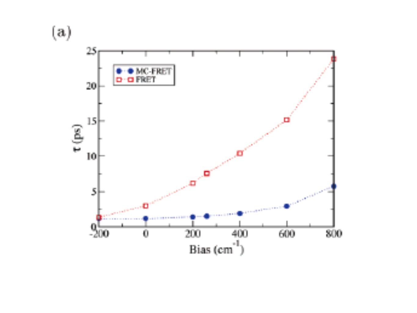
47. How does the B850 coherence effect the B800 -> B850 energy transfer? Compare the energy transfer rate between B800 and B850 using standard Forster theory (FRET) with the energy transfer rate when the coherent states of B850, including disorder, are used (MC- FRET).

49. What happens if we change the relative energies of the B800 and B850 molecular transitions? Jang, Newton and Silbey, JPC (2007)

51. Our calculations suggest that the coherence in the multi-chromophoric aggregate of the B850 band plays a role in keeping the FRET rate from B800 to B850 stable for changes in the relative excitation energies of the B800 Chlorophyls and the B850 Chlorophyls. --- This will have to tested in other aggregates to see if it is general.

52. Conclusions Since we almost always do second order theory, we should try to choose H 0 and V to make the analysis as wide ranging as possible. Coherent and incoherent interactions have been looked at in the context of a unified band and hopping picture. Perhaps we can learn something from that perspective. The interaction between dephasing, population decay, static energetic disorder and coherent interactions, especially at room T have to be explored by a number of methods. In LH2, it is clear that coherence in the electronic states plays a fundamental role in the (~ picoseond) energy transfer processes.