1. Everything You Ever Wanted to Know about Statistics
Prof. Andy Field

2. Aims and Objectives
Know what a statistical model is and why we use them.
The mean
Know what the ‘fit’ of a model is and why it is important.
The standard deviation
Distinguish models for samples and populations
Slide 2

3. The Research Process

4. Whatever the phenomenon we desire to explain, we collect data from the real world to test our hypotheses about the phenomenon.
Testing these hypotheses involves building statistical models of the phenomenon of interest.
Imagine an engineer wishes to build a bridge across a river. That engineer would be pretty daft if she just built any old bridge, because the chances are that it would fall down. Instead, an engineer collects data from the real world: she looks at bridges in the real world and sees what materials they are made from, what structures they use and so on (she might
even collect data about whether these bridges are damaged!). She then uses this information to construct a model.
She builds a scaled-down version of the real-world bridge because it is impractical, not to mention expensive, to build the actual bridge itself. The model may differ from reality in several ways – it will be smaller for a start – but the engineer will try to build a model that best fits the situation of interest based on the data available. Once the model has been built, it can be used to predict things about the real world: for example, the engineer might test whether the bridge can withstand strong winds by placing the model in a wind tunnel. It seems obvious that it is important that the model is an accurate representation of the real world.
Social scientists do much the same thing as engineers: they build models of real-world processes in an attempt to predict how these processes operate under certain conditions. We don’t have direct access to the processes, so we collect data that represent the processes and then use these data to build statistical models (we reduce the process to a statistical model).
We then use this statistical model to make predictions about the real-world
phenomenon. Just like the engineer, we want our models to be as accurate
as possible so that we can be confident that the predictions we make are
also accurate.
However, unlike engineers we don’t have access to the real-world situation
and so we can only ever infer things about psychological, societal,
biological or economic processes based upon the models we build.
If we want our inferences to be accurate then the statistical model we
build must represent the data collected (the observed data) as closely
as possible. The degree to which a statistical model represents the data
collected is known as the fit of the model.

5. Most of the models that we use to describe data tend to be linear models.
Suppose we measured how many chapters of this book a person had read, and then measured their spiritual enrichment.
We could represent these hypothetical data in the form of a scatterplot in which each dot represents an individual’s score on both variables (see section 4.5).
Figure 2.3 shows two versions of such a graph summarizing the pattern of these data with either a straight (left) or curved (right) line.
These graphs illustrate how we can fit different types of models to the same data.
It is always useful to plot your data first: plots tell you a great deal about what models should be applied to data.
If your plot seems to suggest a non-linear model then investigate this possibility.

6. Populations and Samples
The collection of units (be they people, plankton, plants, cities, suicidal authors, etc.) to which we want to generalize a set of findings or a statistical model
Sample
A smaller (but hopefully representative) collection of units from a population used to determine truths about that population
If we take several random samples from the population, each of these samples will give us slightly different results. However, on average, large samples should be fairly similar.

7. The Only Equation You Will Ever Need
Slide 7

8. A Simple Statistical Model
In statistics we fit models to our data (i.e. we use a statistical model to represent what is happening in the real world).
The mean is a hypothetical value i.e. it doesn’t have to be a value that actually exists in the data set.
As such, the mean is simple statistical model.
The mean is the sum of all scores divided by the number of scores.
The mean is also the value from which the (squared) scores deviate least (it has the least error).
One of the simplest models we use in statistics is the mean. Some of you may have trouble thinking of the mean as a model, but in fact it is because it represents a summary of data. The mean is a hypothetical value that can be calculated for any data set, it doesn’t have to be a value that is actually observed in the data set. For example, if we took five statistics lecturers and measured the number of friends that they had, we might find the following data: 1, 3, 4, 3, 2. If we take the mean number of friends, this can be calculated by adding the values we obtained, and dividing by the number of values measured:. Now, we know that it is impossible to have 2.6 friends (unless you chop someone up with a chainsaw and befriend part of their remains, which in practice has proved disturbing) so the mean value is a hypothetical value. As such, the mean is a model that we create to summarise our data.
Slide 8

9. Divide by the number of scores, n:
For example, if we took five statistics lecturers and measured the
number of friends that they had, we might find the following data: 1, 2, 3, 3 and 4. If we take the mean number of friends, this can be calculated by adding the values we obtained, and dividing by the number of values measured:
Collect some data:
1, 3, 4, 3, 2
Add them up:
Divide by the number of scores, n:
Now, we know that it is impossible to have 2.6 friends, unless you chop them up.
Slide 9

10. Measuring the ‘Fit’ of the Model
The mean is a model of what happens in the real world: the typical score.
It is not a perfect representation of the data.
How can we assess how well the mean represents reality?
Slide 10

11. A Perfect Fit
Rating (out of 5)
Rater
Slide 11

12. Calculating ‘Error’
A deviation is the difference between the mean and an actual data point.
Deviations can be calculated by taking each score and subtracting the mean from it:
Slide 12

13. The line representing the mean can be thought of as
our model, and the circles are the observed data.
Vertical lines represent the deviance between the observed data and
our model and can be thought of as the error in the model.
Negative deviances show how the mean underestimates the data and positive
deviances overestimate the data.
Slide 13

14. Use the Total Error?
We could just take the error between the mean and the data and add them.
Score
Mean
Deviation 1
2.6
-1.6 2
-0.6 3
0.4 4
1.4
Total =
There were errors but some of them were positive, some were negative and they have cancelled each other out.
Slide 14

15. Sum of Squared Errors
We could add the deviations to find out the total error.
Deviations cancel out because some are positive and others negative.
Therefore, we square each deviation.
If we add these squared deviations we get the sum of squared errors (SS).
Slide 15

16. Score Mean Deviation Squared Deviation1
2.6
-1.6
2.56 2
-0.6
0.36 3
0.4
0.16 4
1.4
1.96
Total
5.20
Slide 16

17. Variance
The sum of squares is a good measure of overall variability, but is dependent on the number of scores.
We calculate the average variability by dividing by the number of scores (n).
This value is called the variance (s2).
Why N-1, not N? It is a degree of freedom => next slide
Slide 17

18. In statistical terms the degrees of freedom relate to the number of observations that are free to vary.
If we take a sample of four observations from a population, then these four scores are free to vary in any way (they can be any value).
However, if we then use this sample of four observations to calculate the standard deviation of the population, we have to use the mean of the sample as an estimate of the population’s mean => we hold one parameter constant.
Say that the mean of the sample was 10;
then we assume that the population mean is 10 also and we keep this value constant.
With this parameter fixed, can all four scores from our sample vary?
The answer is no, because to keep the mean constant only three values are free to vary.
For example, if the values in the sample were 8, 9, 11, 12 (mean = 10) and we changed three of
these values to 7, 15 and 8, then the final value must be 10 to keep the mean constant. Therefore, if we hold one parameter constant then the degrees of freedom must be one less than the sample size.
This fact explains why when we use a sample to estimate the standard deviation of a population, we have to divide the sums of squares by N − 1 rather than N alone.

19. Standard Deviation
The variance has one problem: it is measured in units squared.
This isn’t a very meaningful metric so we take the square root value.
This is the standard deviation (s).
Slide 19

20. Important Things to Remember
The sum of squares, variance, and standard deviation represent the same thing:
The ‘fit’ of the mean to the data
The variability in the data
How well the mean represents the observed data
Error
Slide 20

21. Same Mean, Different SD
A large standard deviation (relative to the mean) indicates that the data points are distant from the mean (i.e., the mean is not an accurate representation of the data).
A standard deviation of 0 would mean that all of the scores were the same.
Figure 2.5 shows the overall ratings (on a 5-point scale) of two lecturers after each of five different lectures.
Both lecturers had an average rating of 2.6 out of 5 across the lectures.
However, the first lecturer had a standard deviation of 0.55 (relatively small compared to the mean).
It should be clear from the graph that ratings for this lecturer were consistently close to the mean rating.
There was a small fluctuation, but generally his lectures did not vary in popularity.
As such, the mean is an accurate representation of his ratings. The mean is a good fit to the data.
The second lecturer, however, had a standard deviation of 1.82 (relatively high compared to the mean).
The ratings for this lecturer are clearly more spread from the mean; that is, for some lectures he received very high ratings, and for others his ratings were appalling.
Therefore, the mean is not such an accurate representation of his performance because there was a lot of variability in the popularity of his lectures. The mean is a poor fit to the data.
This illustration should make clear why the standard deviation is a measure of how well the mean represents the data.
Slide 21

22. The SD and the Shape of a Distribution
As well as telling us about the accuracy of the mean as a model of our data set, the variance and standard deviation also tell us about the shape of the distribution of scores.
As such, they are measures of dispersion like those we encountered in section
If the mean represents the data well then most of the scores will cluster close to the mean and the resulting standard deviation is small relative to the mean.
When the mean is a worse representation of the data, the scores cluster more widely around the mean (think back to Figure 2.5) and the standard deviation is larger.
Figure 2.6 shows two distributions that have the same mean (50) but different standard deviations.
One has a large standard deviation relative to the mean (SD = 25) and this results in a flatter distribution that is more spread out, whereas the other has a small standard deviation relative to the mean (SD = 15) resulting in a more pointy distribution in which scores close to the mean are very frequent but scores further from the mean become increasingly infrequent.
The main message is that as the standard deviation gets larger, the distribution gets fatter.
This can make distributions look platykurtic or leptokurtic when, in fact, they are not.

23. 2.4.3. Expressing the mean as a model
The discussion of means, sums of squares and variance may seem a sidetrack from the initial point about fitting statistical models, but it’s not: the mean is a simple statistical model that can be fitted to data.
Everything in statistics essentially boils down to one equation:
This just means that the data we observe can be predicted from the model we choose to fit to the data plus some amount of error.
When I say that the mean is a simple statistical model, then all I mean is that we can replace the word ‘model’ with the word ‘mean’ in that equation.
If we return to our example involving the number of friends that statistics lecturers have and look at lecturer 1, for example, we observed that they had one friend and the mean of all lecturers was 2.6.
So, the equation becomes:
From this we can work out that the error is 1 − 2.6, or −1.6.
If we replace this value in the equation we get 1 = 2.6 − 1.6 or 1 = 1.
Although it probably seems like I’m stating the obvious, it is worth bearing this general equation in mind throughout this book because if you do you’ll discover that most things ultimately boil down to this one simple idea!
Likewise, the variance and standard deviation illustrate another fundamental concept:
how the goodness of fit of a model can be measured.
If we’re looking at how well a model fits the data (in this case our model is the mean) then we generally look at deviation from the model = sum of squared error:
Put another way, we assess models by comparing the data we observe to the model we’ve fitted to the data, and then square these differences.
Again, you’ll come across this fundamental idea time and time again throughout this book.

24. Samples vs. Populations
Mean and SD describe only the sample from which they were calculated.
Population
Mean and SD are intended to describe the entire population (very rare in practice).
Sample to Population:
Mean and SD are obtained from a sample, but are used to estimate the mean and SD of the population (very common in practice).
Slide 24

25. Standard deviation shows how well the mean represents the sample data, but data come from samples because we don’t have access to the entire population. Different samples will differ slightly => important to know how well a particular sample represents the population. This is where we use the standard error
Samples are used to estimate the behavior in a population. Imagine that we were interested in the ratings of all lecturers (so lecturers in general were the population). We could take a sample from this population -- one of many possible samples.
If we take several samples from the same population, then each sample has its own mean, and some of these sample means will be different.
Imagine that we could get ratings of all lecturers on the planet and that, on average, the rating is 3 (this is the population mean, µ).
Of course, we can’t collect ratings of all lecturers, so we use a sample.
For each of these samples we can calculate the average, or sample mean.
Let’s imagine we took nine different samples (as in the diagram); you can see that some of
the samples have the same mean as the population but some have different means:
the first sample of lecturers were rated, on average, as 3,
but the second sample were, on average, rated as only 2.
This illustrates sampling variation: that is, samples will vary because they contain different
members of the population; a sample that by chance includes some very good lecturers will
have a higher average than a sample that, by chance, includes some awful lecturers!
We can actually plot the sample means as a frequency distribution, or histogram, just like
I have done in the diagram. This distribution shows that there were three samples that
had a mean of 3, means of 2 and 4 occurred in two samples each, and means of 1 and 5
occurred in only one sample each. The end result is a nice symmetrical distribution known
as a sampling distribution. A sampling distribution is simply the frequency distribution of
sample means from the same population.
In theory you need to imagine that we’re taking hundreds or thousands of samples to construct a sampling distribution, but I’m just using nine to keep the diagram simple.
The sampling distribution tells us about the behavior of samples from the population, and you’ll notice that it is centred at the same value as the mean of the population (i.e., 3).
This means that if we took the average of all sample means we’d get the value of the population mean.
If we knew the accuracy of that average we’d know something about how likely it is that a given sample is representative of the population.
If you were to calculate the standard deviation between sample means then this
too would give you a measure of how much variability there was between the means of
different samples.

26. The standard deviation of sample means is known as the standard error of the mean (SE).
Therefore, the standard error could be calculated by taking the difference between each sample mean and the overall mean, squaring these differences, adding them up, and then dividing by the number of samples.
Finally, the square root of this value would need to be taken to get the standard deviation of sample means, the standard error.
Of course, in reality we cannot collect hundreds of samples and so we rely on approximations of the standard error.
Luckily for us some exceptionally clever statisticians have demonstrated that as samples get large (usually defined as greater than 30), the sampling distribution has a normal distribution with a mean equal
to the population mean, and a standard deviation of:
This is known as the Central Limit Theorem (CLT) and it is useful in this context
because it means that if our sample is large we can use the above equation to
approximate the standard error (because, remember, it is the standard
deviation of the sampling distribution).
When the sample is relatively small (fewer than 30) the sampling distribution
has a different shape, known as a t-distribution, which we’ll come back to later.
The standard error is the standard deviation of sample means.
As such, it is a measure of how representative a sample is likely to be of the population.
A large standard error (relative to the sample mean) means that there is a lot of variability
between the means of different samples and so the sample we have might not be
representative of the population.
A small standard error indicates that most sample means are similar to the population
mean and so our sample is likely to be an accurate reflection of the population.

27.  = 10
M = 8
M = 10
M = 9
M = 11
M = 12
Population

28. Confidence intervals
Remember that usually we’re interested in using the sample mean as an estimate of the value in the population.
We’ve just seen that different samples will give rise to different values of the mean, and we can use the standard error to get some idea of the extent to which sample means differ.
A different approach to assessing the accuracy of the sample mean as an estimate of the mean in the population is to calculate boundaries within which we believe the true value of the mean will fall - CI
Let’s imagine an example: Domjan, Blesbois, and Williams (1998) examined the learnt release of sperm in Japanese quail.
The basic idea is that if a quail is allowed to copulate with a female quail in a certain context (an experimental chamber) then this context will serve as a cue to copulation and this in turn will affect semen release (although during the test phase the poor quail were tricked into copulating with a terry cloth with an embalmed female quail head stuck on top).
If we look at the mean amount of sperm released in the experimental chamber, there is a true mean (the mean in the population); let’s imagine it’s 15 million sperm.
Now, in our actual sample, we might find the mean amount of sperm released was 17 million.
Because we don’t know the true mean, we don’t really know whether our sample value of 17 million is a good or bad estimate of this value.
What we can do instead is use an interval estimate: we use our sample value as the mid-point, but
set a lower and upper limit as well.
So, we might say, we think the true value of the mean sperm release is somewhere between 12 million and 22 million spermatozoa (note that 17 million falls exactly between these values).
Of course, in this case the true value (15 million) does falls within these limits.
However, what if we’d set smaller limits, what if we’d said we think the true value falls between 16 and 18 mil - does not contain the true value of the mean.

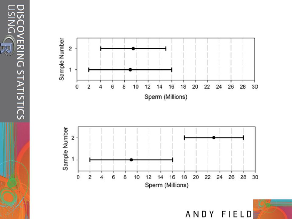
29. Let’s repeat experiment 50 times using different samples.
Each time you did the experiment again you constructed an interval around the sample mean as I’ve just described.
Figure 2.8 shows this scenario: the circles represent the mean for each sample with the lines sticking out of them representing the intervals for these means.
The true value of the mean (the mean in
the population) is 15 million and is shown by a vertical line.
The first thing to note is that the sample means are different from the true mean (this is because of sampling variation as
described in the previous section). Second, although most of the intervals do contain the true mean (they cross the vertical line, meaning that the value of 15 million spermatozoa falls somewhere between the lower and upper boundaries), a few do not.
Slide 29

31. Test Statistics
A statistic for which the frequency of particular values is known.
Observed values can be used to test hypotheses.

32. One- and Two-Tailed Tests

33. Type I and Type II Errors
Type I error
occurs when we believe that there is a genuine effect in our population when, in fact, there isn’t.
The probability is the α-level (usually .05)
Type II error
occurs when we believe that there is no effect in the population when, in reality, there is.
The probability is the β-level (often .2)

34. What Does Statistical Significance Tell Us?
The importance of an effect?
No, significance depends on sample size.
That the null hypothesis is false?
No, it is always false.
That the null hypothesis is true?
No, it is never true.

35. An effect size is a standardized measure of the size of an effect:
Effect Sizes
An effect size is a standardized measure of the size of an effect:
Standardized = comparable across studies
Not (as) reliant on the sample size
Allows people to objectively evaluate the size of observed effect.
Andy Field
PG Stats

36. Effect Size Measures r = .1, d = .2 (small effect):
the effect explains 1% of the total variance.
r = .3, d = .5 (medium effect):
the effect accounts for 9% of the total variance.
r = .5, d = .8 (large effect):
the effect accounts for 25% of the variance.
Beware of these ‘canned’ effect sizes though:
The size of effect should be placed within the research context.
Andy Field
PG Stats

37. Effect Size Measures
There are several effect size measures that can be used:
Cohen’s d
Pearson’s r
Glass’ Δ
Hedges’ g
Odds ratio/risk rates
Pearson’s r is a good intuitive measure
Oh, apart from when group sizes are different …
Andy Field
PG Stats