1. Materials for Lecture 15 Financial Models Finish Scenario Ranking Lecture New Material for Lecture 15 –Read Chapters 13 and 14 –Lecture 15 Pro Forma.xls –Lecture 15 Fin Risk Manager.xls –Lecture 15 Farm Simulator.xls –Lecture 15 Income Taxes.xls

2. 3. Stochastic Efficiency (SERF) Stochastic Efficiency with Respect to a Function (SERF) calculates the certainty equivalent for risky alternatives at 25 different RAC levels –Compare CE of all risky alternatives at each RAC level –Scenario with the highest CE for the DM’s RAC is the preferred scenario –Summarize the CE results for possible RACs in a chart –Identify the “efficient set” based on the highest CE within a range of RACs Efficient Set –This is utility shorthand for saying the risky alternative(s) that is (are) the most preferred

3. Ranking Scenarios with Stochastic Efficiency (SERF) SERF requires an assumption about the decision makers’ utility function and like SDRF uses a range of RAC’s SERF ranks risky strategies based on expected utility which is expressed as CE at the DM’s RAC level Simetar includes SERF and calculates a table of CE’s over a range of RAC values from the LRAC to the URAC and develops a chart for ranking alternatives

4. Ranking Scenarios with SERF SERF results point out the reason that SDRF produces inconsistent rankings –SDRF only uses the minimum and maximum RACs –The efficient set (ranking) can differ from minimum the RAC to the maximum RAC –Changing the RACs and re-running SDRF can be slow SERF can show the actual RAC where the decision maker is indifferent between scenarios (this is the BRAC or breakeven risk aversion coefficient) The SERF Table is best understood as a chart developed by Simetar

5. Ranking Scenarios with SERF Two examples are presented next The first is for ranking an annual decision using annual net cash income –Uses negative exponential utility function –Lower ARAC = zero –Upper ARAC = 4.0/Wealth The second example is for ranking a multiple year decision using NPV variable –Uses Power Utility function –Lower RRAC = zero –Upper RRAC = 4.001

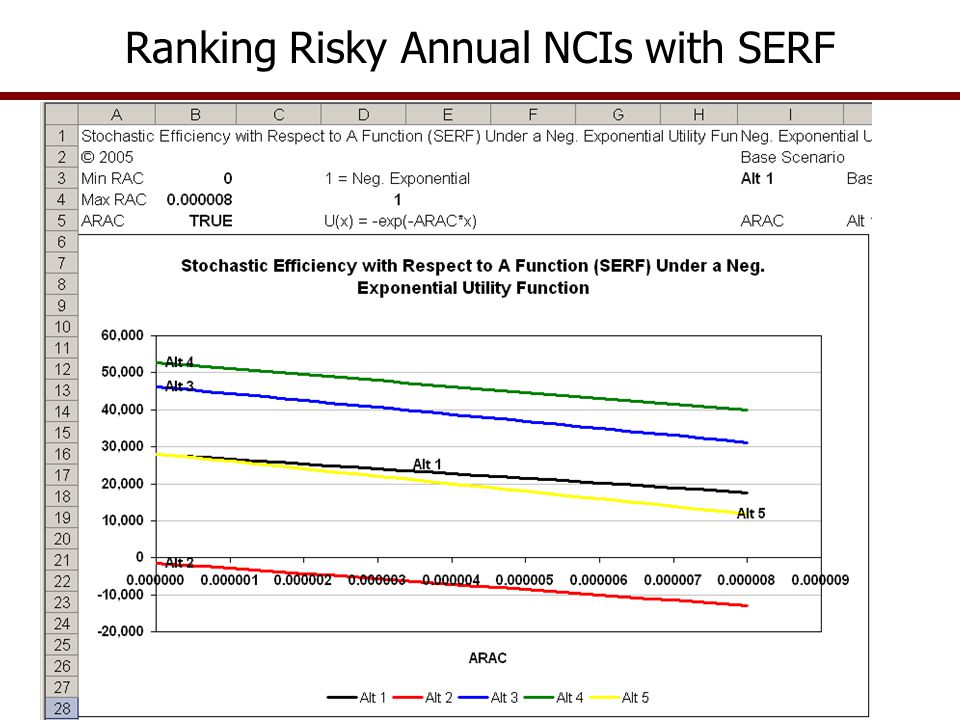
6. Ranking Risky Annual NCIs with SERF

8. Ranking Risky Alternative NPVs with SERF

9. Ranking Risky Alternatives with SERF Interpret the SERF chart as follows –The risky alternative that has the highest CE at a particular RAC is the preferred strategy –Within a range of RACs the risky alternative which has the highest CE line is preferred –If the CE lines cross at that point the DM is indifferent between the two risky alternatives and find a BRAC –If the CE line goes negative, the DM would rather earn nothing than to invest in that alternative –Interpret the rankings within risk aversion intervals RAC = 0 is for risk neutral DM’s RAC = 1 or 1/W is for normal slightly risk aversion DM’s RAC = 2 or 2/W is for moderately risk averse DM’s RAC = 4 or 4/W is for extremely risk averse DM’s

10. Ranking Using Risk Premiums Risk Premium (RP) - calculate the risk premium between each of the scenarios and another scenario. Risk Premiums equals difference between the CE’s for the risky scenarios: RP G to F = CE G – CE F Rank the risky scenarios based on the RPs Advantage is that the full distribution (F(x) and G(x)) of values for the KOV are compared to each other distribution, based on the decision maker’s RAC A wide range of RACs can be tested to allow for a wider range of decision makers given an assumed utility function Base scenario should be the current situation or the scenario picked best by stochastic efficiency (SERF)

11. Ranking Using Risk Premiums Table The RP Table is calculated like the SERF Table using the same range of 25 RACs The user specifies the base scenario; Option 1 was selected for this example Select the scenario that has highest risk premium for the RAC which best defines the decision maker

12. Ranking Using Risk Premiums Risk premiums are presented relative to a base scenario, Alt 1, above Alt 4 is preferred for all risk averse decision makers. Distance between Red line and Base line, $18,347, is how much a risk averse decision maker would pay to move from Alt 2 to Alt 1. Risk averse decision makers prefer Alt 4 to Alt 1 and would pay about $8,000 to gain Alt 4 over Alt 1. Based on the Risk Premium, decision maker would pay to move from Base to Alt 4 Risk Premium decision maker must be paid to accept an inferior scenario

13. Roy (Econometrica, 1952) Select the strategy which minimizes the chance of falling below a critical level of net cash income Rank risky alternatives based on the scenario with the smallest probability of low net cash incomes This is essentially a two light “Stop Light chart” Roy’s Safety First Rule

14. A Roy’s Safety First Rule presented as the probability of NCI i < target each year i With Roy’s Rule, can calculate the probability of a “low” net cash income for two or more consecutive years, as: =IF(AND(NCI 1 <0, NCI 2 <0),1,0) =IF(AND(NCI 2 <0, NCI 3 <0),1,0) =IF(AND(NCI 3 <0, NCI 4 <0),1,0) =IF(AND(NCI 4 <0, NCI 5 <0),1,0) Repeat the =IF(AND()) statement for all years 2-T and summarize the counter variables for all iterations Roy’s probability is sum for all of the =IF(AND()) values divided by (No. Years – 1) * No. Iterations –If 10 years and 500 iterations the denominator is 4,500 representing all possible sample observations that could be 1 Roy’s Safety First Rule

15. The scenario was simulated 100 iterations Net cash income is for 10 years Roy’s values are for 2 consecutive years with negative NCI Roy’s Probability is the sum of the =IF(AND()) counter variables divided by 900, which is = 9 * no. iterations

16. Roy’s Safety First Rule The Stop Light displays the probabilities of having two years of negative NCI in a row, years 1 & 2 or Years 3 & 4, etc. Chart developed from the data in the previous overhead, over all 100 iterations The counter variables can be 0 or 1 so not marginal probabilities and thus no yellow in the Stop Light

17. Multi-Year Financial Models Business decisions often are made based on simple rules –Mean net return (IRR, NPV, etc.) –Worst case and best case –Number of years to payoff debt –Give the business control of its supply chain, etc. These business decisions are inherently multi-year in nature

18. KOVS for a Multi-Year Financial Models –Annual net cash income Probability of negative NCI t –Annual ending cash reserves Probability of negative ending cash t Probability of having to refinance deficits t –Annual net worth (nominal t and real t ) Probability of decreasing RNW relative to BNW –Annual debt to asset ratio Probability of insolvency –NPV summarizes returns over multiple years Probability of positive NPV or P(economic success)

19. Multi-Year Financial Models Common theme or features for multi-year financial models –Input values have annual projections Prices paid and received Annual inflation rates for costs of production Inflation rates for asset values Machinery replacement plans –Management controls are expressed as annual values so, can be strategically managed Assumptions about changing productivity Assumptions about possible structural changes Assumptions about competition and demand Assumptions about beginning cash reserves

20. Multi-Year Financial Models Common set of intermediate calculations –Income Statement Receipts from each source –Total Receipts Cash expenses for each category (non-cash expenses such as depreciation not included here) –Total Cash Expenses Net Cash Income –Cash Flow Statement Net cash income and all other sources of income All cash outflows: taxes, principal payments, owner withdrawals or dividends Ending Cash Reserves –Balance Sheet Assets starting with positive cash balance Liabilities –Including cash flow deficits Net Worth –Financial summary ratios: Debt Asset, PVENW, NPV

21. Multi-Year Financial Models A significant problem can occur with multiple year simulation models –Ending cash reserves can be negative, which causes problems in all three pro forma financial statements What happens if ending cash is negative? –Cash reserves are zero –Must create a short-term liability –Must pay interest for this loan next year –Must repay the short-term loan next year –This is why Ending Cash is a KOV

22. Multi-Year Financial Models Problem of negative ending cash is much greater in agriculture and agribusiness models -- it occurs more often than in non-ag businesses Risk on prices and production greater than for non-ag business interests If you build financial models that do not accommodate this problem, you understate the risk involved with an investment

23. Modeling Negative Cash Flow for Multi-Year Financial Models Modification to the pro forma financials for negative cash flows are simple Change the Income statement –Add an expense for interest paid on cash flow deficit loans – keep it separate from operating interest paid (-5 on Lab Exam!) Change the Cash Flow Statement –Make Beginning Cash equal to Cash Balance in the Balance Sheet (it should be this way but many students make the mistake of making it equal to ending cash t-1 -- -5 on Lab Exam!) –Add a cash outflow to repay the short-term loan borrowed in the previous year to meet a deficit (-5 on Lab Exam!) Change the Balance Sheet –IF() statement for Beginning Cash – that it must be positive or zero (-5 on Lab Exam!) –IF() statement for a Short-Term Liability to have a positive value if ending cash reserve is negative (-5 on Lab Exam!)

26. Multi-Year Financial Models – Income Taxes Income taxes must be considered explicitly Calculate taxable income Taxable Income = Total receipts – total cash expenses - depreciation allowance - deductions Use a tax table to compute taxes due Enter taxes paid in the Cashflow Statement

27. Multi-Year Financial Models – Applications Financial risk management –Analysis of the economic impact of changes in the business plan for a firm on Ability to repay loans on time Ability to remain solvent Ability to earn a satisfactory rate of return on investment –Analysis of alternative marketing schemes that use contracts, futures and options to manage price risk Testing Portfolios –Analysis of alternative combinations of investment instruments (stocks, bonds, land, etc.) –A portfolio of investments is similar to a derivative in the investment world

28. Financial Risk Management A farm level simulation model developed to analyze the financial risk faced by a farm or to appraise a farm in a risky world Input data for initial financial situation of a farm with 10 years of price and yield history providing measures of risk in production and marketing Several financial instruments are available to test the effects of different financial arrangements on firm’s cash flows and ability to repay operating loan and remain current on long- and intermediate-term loans

29. Financial Risk Management

35. Uses of this type of model –Test ability of firm to repay operating debt under alternative assumptions about Other income Family/dividend withdrawal assumptions Machinery replacement plans Re-financing the initial machinery loans Insurance, pricing, and marketing options for the crops Farm program provisions Costs of production including rental rates for land Purchasing land rather than leasing Users of this type of model –Lenders concerned about loan solvency –Borrowers concerned about impacts of growth or adding a family member