1. Distributed Computing
COEN 317
DC5: Time

2. Chapter 11 Time and Global States
Clocks and Synchronization Algorithms
Lamport Timestamps and Vector Clocks
Distributed Snapshots and Termination

3. What Do We Mean By Time? Monotonic increasing
Useful when everyone agrees on it
UTC is Universal Coordinated Time.
NIST operates on a short wave radio frequency WWV and transmits UTC from Colorado.

4. Clock Synchronization
When each machine has its own clock, an event that occurred after another event may nevertheless be assigned an earlier time.

5. Time Time is complicated in a distributed system.
Physical clocks run at slightly different rates – so they can ‘drift’ apart.
Clock makers specify a maximum drift rate  (rho).
By definition
1- <= dC/dt <= 1+ where C(t) is the clock’s time as a function of the real time.

6. Clock Synchronization
The relation between clock time and UTC when clocks tick at different rates.

7. Clock Synchronization
1- <= dC/dt <= 1+
A perfect clock has dC/dt = 1
Assuming 2 clocks have the same max drift rate . To keep them synchronized to within a time interval delta, , they must re-sync every /2 seconds.

8. Cristian’s Algorithm
One of the nodes (or processors) in the distributed system is a time server TS (presumably with access to UTC). How can the other nodes be sync’ed?
Periodically, at least every /2 seconds, each machine sends a message to the TS asking for the current time and the TS responds.

9. Getting the current time from a time server.
Cristian's Algorithm
Getting the current time from a time server.

10. Cristian’s Algorithm
Should the client node simply force his clock to the value in the message??
Potential problem: if client’s clock was fast, new time may be less than his current time, and just setting the clock to the new time might make time appear to run backwards on that node.
TIME MUST NEVER RUN BACKWARDS. There are many applications that depend on the fact that time is always increasing. So new time must be worked in gradually.

11. Cristian’s Algorithm
Can we compensate for the delay from when TS sends the response to T1 (when it is received)?
Add (T1 – T0)/2. If no outside info is available.
Estimate or ask server how long it takes to process time request, say R. Then add (T1 – T0 – R)/2.
Take several measurements and taking the smallest or an average after throwing out the large values.

12. The Berkeley Algorithm
The server actively tries to sync the clocks of a DS. This algorithm is appropriate if no one has UTC and all must agree on the time.
Server “polls” each machine by sending his current time and asking for the difference between his and theirs. Each site responds with the difference.
Server computes ‘average’ with some compensation for transmission time.
Server computes how each machine would need to adjust his clock and sends each machine instructions.

13. The Berkeley Algorithm
The time daemon asks all the other machines for their clock values
The machines answer
The time daemon tells everyone how to adjust their clock

14. Analysis of Sync Algorithms
Cristian’s algorithm: N clients send and receive a message every /2 seconds.
Berkeley algorithm: 3N messages every /2 seconds.
Both assume a central time server or coordinator. More distributed algorithms exist in which each processor broadcasts its time at an agreed upon time interval and processors go through an agreement protocol to average the value and agree on it.

15. Analysis of Sync Algorithms
In general, algorithms with no coordinator have greater message complexity (more messages for the same number of nodes). That’s the price you pay for equality and no-single-point-of-failure.
With modern hardware, we can achieve “loosely synchronized” clocks. This forms the basis for many distributed algorithms in which logical clocks are used with physical clock timestamps to disambiguate when logical clocks roll over or servers crash and sequence numbers start over (which is inevitable in real implementations).

16. Logical Clocks
What do we really need in a “clock”? For many applications, it is not necessary for nodes of a DS to agree on the real time, only that they agree on some value that has the attributes of time.
Attributes of time: X(t) has the sense or attributes of time if it is strictly increasing.
A real or integer counter can be used. A real number would be closer to reality, however, an integer counter is easier for algorithms and programmers. Thus, for convenience, we use an integer which is incremented anytime an event of possible interest occurs.

17. Logical Clocks in a DS
What is important is usually not when things happened but in what order they happened so the integer counter works well in a centralized system.
However, in a DS, each system has its own logical clock, and you can run into problems if one “clock” gets ahead of others. (like with physical clocks)
We need a rule to synchronize the logical clocks.

18. Lamport Clocks Lamport defined the happens-before relation for DS.
A  B means “A happens before B”.
If A and B are events in the same process and A occurs before B then A  B is true.
If A is the event of a message being sent by one process-node and B is the event of that message being received by another process, then then A  B is true. (A message must be sent before it is received).
Happens-before is the transitive closure of 1 and 2. That is, if AB and BC, then AC.
Any other events are said to be concurrent.

19. Events at Three Processes
ab and ac and bf but b and e are incomparable. bf and ef Does e  b?

20. Lamport Clocks Desired properties:
(1) anytime A B , C(A) < C(B), that is the logical clock value of the earlier event is less
(2) the clock value C is increasing (never runs backwards)

21. Lamport Clocks Rules
An event is an internal event or a message send or receive.
The local clock is increased by one for each message sent and the message carries that timestamp with it.
The local clock is increased for an internal event.
When a message is received, the current local clock value, C, is compared to the message timestamp, T. If the message timestamp, T = C, then set the local clock value to C+1. If T > C, set the clock to T+1. If T<C, set the clock to C+1.

22. Lamport Clocks Anytime A B , C(A) < C(B)
However, C(A) < C(B) doesn’t mean A B
(ex: C(e) < C(b) but it is not true that e b)

23. Total Order Lamport Clocks
If you need a total ordering, (distinguish between event 3 on P2 and event 1 on P3) use Lamport timestamps.
Lamport timestamp of event A at node i is (C(A), i)
For any 2 timestamps T1=(C(A),I) and T2=(C(B),J)
If C(A) > C(B) then T1 > T2.
If C(A) < C(B) then T1 < T2.
If C(A) = C(B) then consider node numbers. If I>J then T1 > T2. If I<J then T1 < T2. If I=J then the two events occurred at the same node, so since their clock C is the same, they must be the same event.

24. Total Order Lamport Timestamps
(1,1)
(2,1)
(4,2)
(3,2)
(1,3)
(5,3)
The order will be (1,1), (1,3), (2,1), (3,2) etc

25. Why Total Order?
Database updates need to be performed in the same order at all sites of a replicated database.

26. Exercise: Lamport Clocks
a b c
d e
f g A B C
Assuming the only events are message send and receive, what are the clock values at events a-g?

27. Limitation of Lamport Clocks
Total order Lamport clocks gives us the property if A  B then C(A) < C(B). But it doesn’t give us the property if C(A) < C(B) then AB. (if C(A) < C(B), A and B may be concurrent or incomparable, but never BA).
2, ,1
1, ,2 A1 B2 C3
Lamport timestamp of 2,1 < 3,3 but the events are unrelated
3,3 4,3

28. A and C will never know messages were out of order
Limitation
Also, Lamport timestamps do not detect causality violations. Causality violations are caused by long communications delays in one channel that are not present in other channels or a non-FIFO channel. A B C
A and C will never know messages were out of order

29. Causality Violation
Causality violation example: A gets a message from B that was sent to all nodes. A responds by sending an answer to all nodes. C gets A’s answer to B before it receives B’s original message.
How can B tell that this message is out of order?
Assume one send event for a set of messages A B C

30. Causality: Solution
The solution is vector timestamps: Each node maintains an array of counters.
If there are N nodes, the array has N integers V(N). V(I) = C, the local clock, if I is the designation of the local node.
In general, V(X) is the latest info the node has on what X’s local clock is.
Gives us the property e  f iff ts(e) < ts(f)

31. Vector Timestamps
Each site has a local clock incremented at each event (not according to Lamport clocks) The vector clock timestamp is piggybacked on each message sent. RULES:
Local clock is incremented for a local event and for a send event. The message carries the vector time stamp.
When a message is received, the local clock is incremented by one. Each other component of the vector is increased to the received vector timestamp component if the current value is less. That is, the maximum of the two components is the new value.

32. Vector Timestamps and Causal Violations
C receives message (2,1,0) then (0,1,0)
The later message causally precedes the first message if we define how to compare timestamps right A B C

33. Vector Clock Comparison
VC1 > VC2 if for each component j, VC1[j] >= VC2[j], and for some component k, VC1[k] > VC2[k]
VC1 = VC2 if for each j, VC1[j] = VC2[j]
Otherwise, VC1 and VC2 are incomparable and the events they represent are concurrent 1 2
Clock at point
1= (2,1,0)
2= (2,2,0)
3= (2,1,1)
4= (2,1,2) A B C

34. Vector Clocks

35. Vector Clock Exercise Assuming the only events are send and receive:
What is the vector clock at events a-f?
Which events are concurrent? a
b e
c d f A B C

36. Matrix Timestamps
Matrix timestamps can be used to give each node more information about the state of the other nodes.
Each site keeps a 2 dimensional time table
If Ti[j,k] = v then site i knows that site j is aware of all events at site k up to v
Row x is the view of the vector clock at site x
A’s TT
A B C A B C A B C

37. Matrix Timestamp Example
3 0 0
0 0 0
Node A in previous slide has table
(just after receiving msg & before updating it’s TT)
Node A receives message from C with timestamp
To get A’s new time table:
compare each row in tables component-wise and take the maximum
update A’s row by taking the max of each column
2 0 0
1 2 0
2 2 3
3 2 3
1 2 0
2 2 3

38. Global State
Matrix timestamps is one way of getting information about the distributed system. Another way is to sample the global state.
The Global state is the combination of the states of all the processors and channels at some time which could have occurred.
Because there is no way of recording states at the exact same time at every node, we will have to be careful how we define this.

39. Global State
There are many reasons for wanting to sample the global state “take a snapshot”.
deadlock detection
finding lost token
termination of a distributed computation
garbage collection
We must define what is meant by the state of a node or a channel.

40. Defining Global State
There are N processes P1…Pn. The state of the process Pi is defined by the system and application being used.
Between each pair of processors, Pi and Pj, there is a one-way communications channel Ci,j. Channels are reliable and FIFO, ie, the messages arrive in the order sent. The contents of Ci,j is an ordered list of messages Li,j = (m1, m2, m3…). The state of the channel is the messages in the channel and their order.
Li,j = (m1, m2, …) is the channel from Pi to Pj and m1 (head or front) is the next message to be delivered.

41. Defining Global State
It is not necessary for all processors to be interconnected, but each processor must have at least one incoming channel and one outgoing channel and it must be possible to reach each processor from any other processor (graph is strongly connected). 2 1 4 3

42. Defining Global State
The Global state is the combination of the states of all the processors and channels.
The state of all the channels, L, is the set of messages sent but not yet received.
Defining the state was easy, getting the state is more difficult.
Intuitively, we say that a consistent global state is a “snapshot” of the DS that looks to the processes as if it were taken at the same instant everywhere.

43. Defining Global State
For a global state to be meaningful, it must be one that could have occurred.
Suppose we observe processor Pi (getting state Si) and it has just received a message m from processor Pk. When we observe processor Pk to get Sk, it should have sent m to Pi in order for us to have a consistent global state. In other words, if we get Pk’s state before it sent message m and then get Pi’s state after it received m, we have an inconsistent global state. Pi Pk Pi Pk

44. Consistent Cut
So we say that the global state must represent a consistent cut.
One way of defining a consistent cut is that the observations resulting in the states Si should all occur concurrently (as defined using vector clocks).
Also, a consistent cut is one where all the events before the cut happen-before the ones after the cut or are unrelated (uses “happens-before” relation).

45. Global State
A consistent cut
An inconsistent cut

46. More Cuts

47. Consistent Cuts and LatticesP1 P2 1 2 3 4
A lattice structure can be used to define all the consistent global states. Sjk is the state where process 1 has had j events and process 2 has had k events. Thus, the consistent cut above is S33

48. Lattice of All Consistent States
time P1 P2 1 2 3 4

49. Vector Clocks and Cuts
All events before a consistent cut happen before (or are concurrent with) all events after the cut

50. Distributed Snapshot Algorithms
Snapshot algorithms are used to record a consistent state of the DS.
Snapshots can be used to detect stable states.
Once the system enters a stable state, it will remain in that state (until there is some outside intervention).
Examples of stable states: lost token, deadlock, termination.

51. Algorithm for Distributed Snapshot
Well known algorithm by Chandy and Lamport
Assumes:
Communication channels are reliable, unidirectional and FIFO
There are no failures
The graph of processes is strongly connected.

52. Chandy and Lamport
When instructed, each processor will stop other processing and record its state Pi, send out marker messages and record the sequence of messages arriving on each incoming channel until a marker comes in (this will enable us to get the channel state Ci,j).
At end of algorithm, initiator or other coordinator collects local states and compiles global state.

53. Chandy Lamport Snapshot
Organization of a process and channels for a distributed snapshot

54. Chandy Lamport Snapshot
One processor starts the snapshot by recording his own local state and immediately sends a marker message M on each of its outgoing channels. (This indicates the causal boundary between before the local state was recorded and after). It begins to record all the messages arriving on all incoming channels. When it has received markers from all incoming channels, it is done.
When a processor who was not the initiator receives the marker for the first time, it immediately records its local state, sends out markers on all outgoing channels. It begins recording the received message sequence on all incoming channels other than the one it just received the marker on. When a marker has been received on each incoming channel that is being recorded, the processor is done with its part of the snapshot.

55. Chandy Lamport Snapshot
Process Q receives a marker for the first time and records its local state
Q records all incoming message
Q receives a marker for its incoming channel and finishes recording the state of the incoming channel

56. Node 2 initiates snapshotM
Recorded: a M
State S2 2 2 1 4 b 3 c
Node 2 initiates snapshot

57. Node 2 initiates snapshot
Recorded: M
State S2 2 2 M 1 b 4 3 c
Node 2 initiates snapshot

58. Node 2 initiates snapshot
Recorded:
State S2 2 2 M
State S1 1 1 b 4 4 4
State S4 M d M 3
Node 2 initiates snapshot

59. Snapshot Recorded: State S2 2 2 M State S1 1 1 M d 4 4 4 State S4
L3,2 = b 3 M

60. Snapshot Recorded: State S2 2 2 State S1 1 1 d 4 4 4 State S4 L3,2 = b
L1,2 = empty M
L4,2 = empty

61. Snapshot Recorded: State S2 2 2 State S1 1 1 4 4 4 State S4 M L3,2 = b
L1,2 = empty
L4,2 = empty
State S3
L3,1 = d

62. Snapshot Recorded: State S2 2 2 State S1 1 1 M M 4 4 4 State S4
L3,2 = b 3 3 3
L1,2 = empty
L4,2 = empty
State S3
L3,1 = d

63. Snapshot Recorded: State S2 2 2 2 State S1 1 1 1 4 4 4 State S4
L3,2 = b 3 3 3
L1,2 = empty
L4,2 = empty
State S3
L3,1 = d

64. Chandy Lamport Snapshot2 2 2 1 1 1 4 4 4 3 3 3
Uses O(|E|) messages where E is the number of edges. Time bound is dependent on the topology of the graph.

65. Chandy Lamport is a Consistent Cut1 a M d M M M 2 c M b 3 M M 4

66. Chandy Lamport is a Consistent Cut1 a d 2 c b 3 4

67. Termination detection

68. Termination Detection
Problem: Determine if a distributed computation has terminated. This is difficult because while some nodes look like they are done, a message from a node not yet queried could awaken them to more computations.
Nodes can be organized in a ring – either physically or logically.
Communications are reliable and FIFO.

69. Termination Detection
Each node can be either in active or in passive state.
Only an active node can send messages to other nodes; each message sent is received after some period of time.
After having received a message, a passive node becomes active; the receipt of a message is the only mechanism that triggers a passive node to become active.
For each node, the transition from the active to the passive state may occur "spontaneously".

70. Termination Detection
The state in which all nodes are passive and no messages are on their way is stable: the distributed computation is said to have terminated.
The purpose of the algorithm is to enable one of the nodes, say node 0, to detect that this stable state has been reached. 1 1 2 2 3 3 4 4

71. Termination Detection
The problem is that a node may say it is finished, but then an incoming message “wakes it up” and it begins processing and perhaps sending out more messages waking up more processes. We cannot query them “all at once” and even if we could, we might miss a message in transition.
Here’s more
work
Are you done?
Yes, I’m done 3 3

72. Dijkstra’s TD Algorithm
Every node maintains a counter c. Sending a message increases c by one; the receipt of a message decreases c by one. The sum of all counters thus equals the number of messages pending in the network. 3 1 1

73. Dijkstra’s TD Algorithm
When node 0 initiates a detection probe, it sends a token with a value 0 to node N-1. Every node i keeps the token until it becomes passive; it then forwards the token to node i-1 increasing the token value by c (the message count). 4 1

74. Dijkstra’s TD Algorithm
Every node and also the token has a color (initially all white). When a node receives a message, the node turns black. When a node forwards the token, the node turns white. If a black machine forwards the token, the token turns black; otherwise the token keeps its color. 4 4 1

75. Dijkstra’s TD Algorithm
When node 0 receives the token again, it can conclude termination, if
node 0 is passive and white,
the token is white, and
the sum of the token value and c is 0.
Otherwise, node 0 may start a new probe. 1
From node 1
To node N-1 -1

76. 1 1 2 2 -1

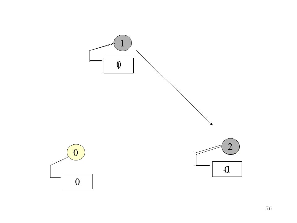
77. 1 1 2 2 -1 -1

78. 1 1 2 2 -1

79. 1 1 1 2 2 -1

80. 1 1 1 1 2 2 -1