1. Lecture 3 (Ch4) Inferences
Research Method
Lecture 3 (Ch4)
Inferences

2. Sampling distribution of OLS estimators
We have learned that MLR.1-MLR4 will guarantee that OLS estimators are unbiased.
In addition, we have learned that, by adding MLR.5, you can estimate the variance of OLS estimators.
However, in order to conduct hypothesis tests, we need to know the sampling distribution of the OLS estimators.

3. To do so, we introduce one more assumption
Assumption MLR.6
　　(i) The population error u is independent of explanatory variables, x1,x2,…,xk, and (ii) u~N(0,σ2).

4. Classical Linear Assumption
MLR.1 through MLR6 are called the classical linear model (CLM) assumptions.
Note that MLR.6(i) automatically satisfies MLR.4(provided E(u)=0 which we always assume), but MLR.4 does not necessarily indicate MLR.6(i). In this sense, MLR.4 is redundant. However, to emphasize that we are making additional assumption, MLR1 through MLR.6 are called CLM assumptions.

5. Conditional on X, we have
Theorem 4.1
Conditional on X, we have
and
Proof: See the front board

6. Hypothesis testing Consider the following multiple linear regression.
y=β0+β1x1+β2x2+….+βkxk+u
Now, I present a well known theorem.

7. Theorem 4.2: t-distribution for the standardized estimators.
Under MLR1 through MLR6 (CLM assumptions) we have
This means that the standardized coefficient follows t-distribution with n-k-1 degree of freedom.
Proof: See the front board.

8. One-sided test One sided test has the following form
The null hypothesis: H0: βj=0
The alternative hypothesis: H1: βj>0

9. Set the significance level . Typically, it is set at 0.05.
Test procedure.
Set the significance level . Typically, it is set at 0.05.
Compute the t-statistics under the H0. that is
Note: Under H0, βj=0, so this simplified to this.

10. 3. Find the cutoff number  This cutoff number is illustrated below.
T-distribution with n-k-1
degree of freedom
tn-k-1,α
The cutoff number.
4. Reject the null hypothesis if the t-statistic falls in the rejection region. This is illustrated in the next page.

11. The illustration of the rejection decision.
T-distribution with n-k-1
degree of freedom
tn-k-1,α
Rejection region.
(Reject H0)
If t-statistic falls in the rejection region, you reject the null hypothesis. Otherwise, you fail to reject the null hypothesis.

12. Note, if you want to test if βj is negative, you have the following null and alternative hypotheses,
H0: βj=0
H1: βj<0
Then the rejection region will be on the negative side. Nothing else changes.
-tn-k-1,α
Rejection region.

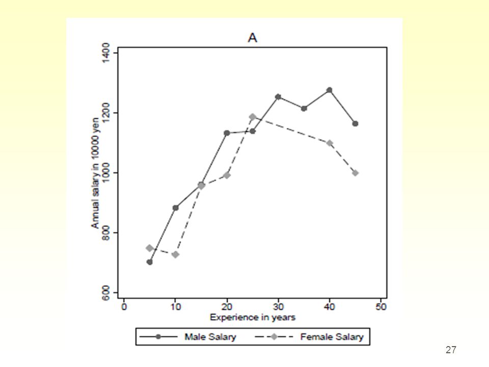
13. Example
The next slide shows the estimated result of the log salary equation for 338 Japanese economists. (Estimation is done by STATA.)
The estimated regression is
Log(salary)=β0+β1(female)+ δ(other variables)+u

14. SSE
T-statistics
SSR
SST

15. Q1. Test if female salary is lower than male salary at 5% significance level (i.e., =0.05). That is test,
H0: β1=0
H1: β1<0

16. Two sided test Two sided test has the following form
The null hypothesis: H0: βj=0
The alternative hypothesis: H1: βj≠0

17. Set the significance level . Typically, it is set at 0.05.
Test procedure.
Set the significance level . Typically, it is set at 0.05.
Compute the t-statistics under the H0. that is
Note: Under H0, βj=0, so this simplified to this.

18. 3. Find the cutoff number . This cutoff number is illustrated below.
T-distribution with n-k-1
degree of freedom
-tn-k-1,α/2
tn-k-1,α/2
The cutoff number.
Rejection region
4. Reject the null hypothesis if t-statistic falls in the rejection region above.

19. When you reject the null hypothesis βj≠0 using two sided test, we say that the variable xj is statistically significant.

20. Exercise Consider again the following regression
Log(salary)=β0+β1(female)+ δ(other variables)+u
This time, test if female coefficient is equal to zero or not using two sided test at the 5% significance level. That is, test
H0: β1=0
H1: β1≠0

21. SSE
SSR
SST

22. The p-value
The p-value is the minimum level of the significance level ( ) at which, the coefficient is statistically significant.
STATA program automatically compute this value for you.
Take a look at the salary regression again.

23. SSE
SSR
P-values
SST

24. Other hypotheses about βj
You can test other hypotheses, such as βj=1 or βj=-1. Consider the null hypothesis
β j=a
Then, all you have to do is to compute t-statistics as
Then other test procedure is exactly the same.

25. Consider the following regression results.
Log(crime)= log(enroll)
(1.03) (0.11)
n=97, R2=0.585
Now, test if coefficient for log(enroll) is equal to 1 or not using two sided test at the 5% significance level.

26. The F-test Testing general linear restrictions
You are often interested in more complicated hypothesis testing.
First, I will show you some examples of such tests using the salary regression example.

28. Example 1: Modified salary equation.
Log(salary)=β0+β1(female)
+β2(female)×(Exp>20)
+β(other variables)+u
Where (Exp>20) is the dummy variable for those with experience greater than 20 years.
Then, it is easy to show that gender salary gap among those with experience greater than 20 years is given by β1+β2.
Then you want to test the following
H0: β1+β2=0 H1: β1+β2≠0

29. Example 2: More on modified salary equation.
Log(salary)=β0+β1(female)
+β2(female)×(Exp)
+β(other variables)+u
Where exp is the years of experience.
Then, if you want to show if there is a gender salary gap at experience equal to 5, you test
H0: β1+5*β2=0 H1: β1+5*β2≠0

30. Example 3: The price of houses.
Log(price)=β0 +β1(assessed price)
+β2(lot size)
+β3(square footage)
+β4(# bedrooms)
Then you would be interested in
H0: β1=1, β2=0, β3=0, β4=0
H1: H0 is not true.
Note in this case, there are 4 equations in H0.

31. The procedure for F-test
Linear restrictions are tested using F-test. The general procedure can be explained using the following example.
Y= β0+β1x1+β2x2+β3x3+β4x4+u (1)
Suppose you want to test
H0: β1=1, β2=β3, β4=0
H1: H0 is not true

32. Step 1: Plug in the hypothetical values of coefficient given by H0 in the equation 1. Then you get
Y= β0+1*x1+β2x2+β2x3+0*x4 +u
(Y-x1)= β0+β2(x2+x3)+u (2)
(2) Is called the restricted model. On the other hand, the original equation (1) is called the unrestricted model.

33. In the restricted model, the dependent variable is (Y-x1)
In the restricted model, the dependent variable is (Y-x1). And now, there is only one explanatory variable, which is (x2+x3).
Now, I can describe the testing procedure.

34. Step 3: Compute the F-statistics as
Step 1: Estimate the unrestricted model (1), and compute SSR. Call this SSRur.
Step 2: Estimate the restricted model (2), and compute SSR. Call this SSRr.
Step 3: Compute the F-statistics as
Where q is the number of equations in H0.
q = numerator degree of freedom
(n-k-1) =denominator degree of freedom

35. Step5: Set the significance level . (Usually, it is set at 0.05)
It is know that F statistic follows the F distribution with degree of freedom (q,n-k-1). That is;
F~Fq,n-k-1
Step5: Set the significance level . (Usually, it is set at 0.05)
Step 6. Find the cutoff value c, such that P(Fq,n-k-1>c)= . This is illustrated in the next slide.
Numerator degree of freedom
Denominator degree of freedom

36. Step 7: Reject if F stat falls in the rejection region.
The density of Fq,n-k-1 1- c
Rejection region
The cutoff points can be found in the table in the next slide.

37. Copyright © 2009 South-Western/Cengage Learning

38. Example
Log(salary)=β0+β1(female) +β2(female)×(Exp>20) + δ(other variables)+u -----(1) Now, let us test the following H0: β1+β2=0 H1: β1+β2≠0

39. Then, restricted model is
Log(salary)=β0
+β1[(female)-(female)×(Exp>10)]
+β(other variables)+u (2)
The following slides show the estimated results for unrestricted and restricted models.

40. The unrestricted model
SSRur

41. Restricted model.
SSRr
Female –Female*(Exp>20)

42. Since we have only one equation in H0, q=1
Since we have only one equation in H0, q=1. And you can see that (n-k-1)=( )=325
F=[( )/1]/[ /325]
=0.0068
The cutoff point at 5% significance level is 3.84.
Since F-stat does not falls in the rejection, we fail to reject the null hypothesis. In other words, we did not find evidence that there is a gender gap among those with experience greater than 20 years.

43. Copyright © 2009 South-Western/Cengage Learning

44. In fact, STATA does F-test automatically.
After estimation, type this command

45. F-test for special case The exclusion restrictions
Consider the following model
Y= β0+β1x1+β2x2+β3x3+β4x4+u (1)
Often you would like to test if a subset of coefficients are all equal to zero. This type of restriction is called `the exclusion restrictions’.

46. Suppose you want to test if β2,β3,β4 are jointly equal to zero
Suppose you want to test if β2,β3,β4 are jointly equal to zero. Then, you test
H0 : β2=0, β3=0, β4=0
H1: H0 is not true.

47. Y= β0+β1x1+β2x2+β3x3+β4x4+u -------(1) Y= β0+β1x1 +u -------(2)
In this special type of F-test, the restricted and unrestricted equations look like
Y= β0+β1x1+β2x2+β3x3+β4x4+u (1)
Y= β0+β1x u (2)
In this special case, F statistic has the following representation
Proof: See the front board.

48. When we reject this type of null hypothesis, we say x2, x3 and x4 are jointly significant.

49. Example of the test of exclusion restrictions
Suppose you are estimating an salary equations for baseball players.
Log(salary)=β0 + β1(years in league)
+β2(average games played)
+β3(batting average)
+β4(homeruns)
+β5(runs batted) +u

50. Do batting average, homeruns and runs batted matters for salary after years in league and average games played are controlled for? To answer to this question, you test
H0: β3=0, β4=0, β5=0
H1: H0 is not true.

51. Unrestricted model
Variables
Coefficient
Standard errors
Years in league
0.0689***
0.0121
Average games played
0.0126***
0.0026
Batting average
0.0011
Homeruns
0.0144
0.016
Runs batted
0.108
0.0072
Constant
11.19***
0.29
# obs
353
R squared
0.6278
SST
As can bee seen, batting average, homeruns and runs batted do not have statistically significant t-stat at the 5% level.

52. The F stat is F=[(198.311-181.186)/3]/[181.186/(353-5-1)]=10.932
Restricted model
Variables
Coefficient
Standard errors
Years in league
0.0713***
0.0125
Average games played
0.0202***
0.0013
Constant
11.22***
0.11
# obs
353
R squared
0.5971
SST
The F stat is
F=[( )/3]/[ /( )]=10.932
The cutoff number of about So we reject the null hypothesis at 5% significance level. This is an reminder that even if each coefficient is individually insignificant, they may be jointly significant.