1. Ad Hoc and Wireless Sensor Network Wireless Computer Communications Min-Xiou Chen

2. Mobile Ad Hoc Networks (MANET)  Formed by wireless hosts which may be mobile  Without (necessarily) using a pre-existing infrastructure  Routes between nodes may potentially contain multiple hops  May need to traverse multiple links to reach a destination  Mobility causes route changes

3. Variations  Fully Symmetric Environment  all nodes have identical capabilities and responsibilities  Asymmetric Capabilities  transmission ranges and radios may differ  battery life at different nodes may differ  processing capacity may be different at different nodes  speed of movement  Asymmetric Responsibilities  only some nodes may route packets  some nodes may act as leaders of nearby nodes (e.g., cluster head)

4. Variations (Cont.)  Traffic characteristics may differ in different ad hoc networks  bit rate  timeliness constraints  reliability requirements  unicast / multicast / geocast  host-based addressing / content-based addressing / capability-based addressing  May co-exist (and co-operate) with an infrastructure-based network

5. Variations (Cont.)  Mobility patterns may be different  people sitting at an airport lounge  New York taxi cabs  kids playing  military movements  personal area network  Mobility characteristics  Speed  Predictability  direction of movement  pattern of movement  uniformity (or lack thereof) of mobility characteristics among different nodes

6. Why Ad Hoc Networks ?  Ease of deployment  Speed of deployment  Decreased dependence on infrastructure

7. Many Applications  Personal area networking  cell phone, laptop, ear phone, wrist watch  Military environments  soldiers, tanks, planes  Civilian environments  taxi cab network  meeting rooms  sports stadiums  boats, small aircraft  Emergency operations  search-and-rescue  policing and fire fighting

8. Challenges  Limited wireless transmission range  Broadcast nature of the wireless medium  Hidden terminal problem  Packet losses due to transmission errors  Mobility-induced route changes  Mobility-induced packet losses  Battery constraints  Potentially frequent network partitions  Ease of snooping on wireless transmissions (security hazard)

9. Flooding for Data Delivery SD P P P P P P P P P P P D S broadcasts data packet P to all its neighbors Each node receiving P forwards P to its neighbors Sequence numbers used to avoid the possibility of forwarding the same packet more than once Node D does not forward the packet

10. Flooding for Data Delivery: Advantages  Simplicity  May be more efficient than other protocols when rate of information transmission is low enough that the overhead of explicit route discovery/maintenance incurred by other protocols is relatively higher  this scenario may occur, for instance, when nodes transmit small data packets relatively infrequently, and many topology changes occur between consecutive packet transmissions  Potentially higher reliability of data delivery  Because packets may be delivered to the destination on multiple paths

11. Flooding for Data Delivery: Disadvantages  Potentially, very high overhead  Data packets may be delivered to too many nodes who do not need to receive them  Potentially lower reliability of data delivery  Flooding uses broadcasting -- hard to implement reliable broadcast delivery without significantly increasing overhead  Broadcasting in IEEE 802.11 MAC is unreliable  In our example, nodes J and K may transmit to node D simultaneously, resulting in loss of the packet  in this case, destination would not receive the packet at all

12. Why is Routing in MANET different ?  Host mobility  link failure/repair due to mobility may have different characteristics than those due to other causes  Rate of link failure/repair may be high when nodes move fast  New performance criteria may be used  route stability despite mobility  energy consumption

13. Changes in network  Number of nodes  Topology  Connectivity  Mobility  Battery power  Heterogeneousness

14. Solution models  Proactive protocols  Reactive protocols  Position-aware protocols  Clustering protocols  Cooperation between protocols

15. Proactive protocols  DSDV, STAR, WRP,...  Propagate routing information before the routes are needed  Possible to have multiple routes for one destination  Lots of signaling traffic  All of the routes may never be used

16. Table-driven, Proactive  Uses periodic route updates to maintain routing tables  Can either be link state or distance vector  Mobility is treated as link change  Drawbacks: Inefficient if there is few demands for routes, and instability if there is high mobility

17. Reactive protocols  AODV, DSR, TORA,...  New nodes are added when needed  Introduce extra latency  Disappearing routes take time to expire  May actually cause more signaling if expiration times are shortened

18. On demand, Reactive  No periodic route updates  Find route when needed by the source node  Caching will help to improve the performance  Advantages: power and bandwidth efficient  Disadvantages: sometimes longer delay

19. Position-aware protocols  GPSR, GRA, ABR,...  Additional location-dependent metrics  Geographic positioning (GPSR, GRA)  Associativity (ABR)  Signal stability (SSA)  Reduce network-wide signaling

20. Hierarchical / Clustering protocols  ZRP, CBR, FSR, LANMAR,...  Avoid drastic network-wide changes  May use hybrid design  Small clusters converge fast

21. Cooperation between different protocols  What if a network comes into contact with another one?

22. Hybrid of Proactive and Reactive  Compromised Method  Reduce disadvantages and promote advantages  On theory better but IMHO it’s a bit too complicated and “smart”, the rule of the real world is “The simpler the better.”

23. Considerations of routing protocol design  Can be adapted to ever changing topology  Low delay  Low power consumption  High throughput (bandwidth)  High QoS

24. Flooding of Control Packets  Many protocols perform (potentially limited) flooding of control packets, instead of data packets  The control packets are used to discover routes  Discovered routes are subsequently used to send data packet(s)  Overhead of control packet flooding is amortized over data packets transmitted between consecutive control packet floods

25. DSDV: Destination Sequence Distance Vector Routing  IBM 1996, simulated but not implemented  Uses modified Bellman-Ford Algorithm, distance vector based, table driven  Route settling time and route may not converge  Sequence number derived from dest. node is used to keep the routing table up- to-date

26. DSDV: Example  MH4 FW TABLE  Dest. Next_Hop Metric Seq._No. Install Stable_Data  MH4 ADV. RT. TABLE  Dest. Metric Seq._No.  MH1 move to the vicinity of MH5 and trigger a broadcast  Routing Update, with increased sequence number in routing table MH4 MH2 MH3 MH5 MH1

27. DSR: Dynamic Source Routing  CMU 1996, simulated and implemented in 1999  An extension of IP, it uses options field in IP  Two phases: routing discovery and routing maintenance  Caching and other features are used

28. DSR  When node S wants to send a packet to node D, but does not know a route to D, node S initiates a route discovery  Source node S floods Route Request (RREQ)  Each node appends own identifier when forwarding RREQ

29. Flooding RREQ S D 3 4 10 572 1 8 9 6 RREQ{} RREQ{1} RREQ{2} RREQ{2,3} RREQ{1,4} RREQ{2,3,5} RREQ{2,3,5,7}

30. Route Discovery in DSR  Destination D on receiving the first RREQ, sends a Route Reply (RREP)  RREP is sent on a route obtained by reversing the route appended to received RREQ  RREP includes the route from S to D on which RREQ was received by node D

31. Send Back RREP S D 3 4 10 572 1 8 9 6 RREP{2,3,5,7}

32. Route Reply in DSR  RREP can be sent only if links are guaranteed to be bi-directional  To ensure this, RREQ should be forwarded only if it received on a bi-directional link  If unidirectional (asymmetric) links are allowed, then RREP may need a route discovery for S from node D  If IEEE 802.11 MAC is used to send data, then links have to be bi-directional (since Ack is used)

33. DSR  Node S on receiving RREP, caches the route included in the RREP  When node S sends a data packet to D, the entire route is included in the packet header  hence the name source routing  Intermediate nodes use the source route included in a packet to determine to whom a packet should be forwarded

34. DSR Routing Maintenance  Topology: A->B->CxD E  Suppose A wants to send a packet to E, it first sent it to B according to the source routing table, and must receive a receipt from B to confirm the success of sending.  B also needs a receipt from C.  If the link from C to D is broken, C sends back link error message to B, and B to A.  A should search its cache to see if there is another route available to E, otherwise, it needs to initiate a new route discovery session.

35. DSR: Advantages  Routes maintained only between nodes who need to communicate  reduces overhead of route maintenance  Route caching can further reduce route discovery overhead  A single route discovery may yield many routes to the destination, due to intermediate nodes replying from local caches

36. DSR: Disadvantages  Packet header size grows with route length due to source routing  Flood of route requests may potentially reach all nodes in the network  Care must be taken to avoid collisions between route requests propagated by neighboring nodes  insertion of random delays before forwarding RREQ  Increased contention if too many route replies come back due to nodes replying using their local cache  Route Reply Storm problem  Reply storm may be eased by preventing a node from sending RREP if it hears another RREP with a shorter route

37. Ad hoc On-Demand Distance Vector (AODV)  允許 mobile nodes 很快的獲得許多路徑到 達它所想要到達的目的地  不要求這些 mobile nodes 在沒有 active communication 去維護這些到目的端的路 徑  允許 mobile nodes 當 link breakages 和網路 拓樸有所改變的時候，能夠快速的去回應， 並且去作一些應對的措施。

38. AODV routing protocol  1. 當 mobile node 發送的 packet 在 routing table 找不到適合的路徑可以到達 Destination node  廣播 Route Requests (RREQs) 去找尋到達 destination node 的新路徑。  2. 當 RREQs 的訊息到達它所指定的 destination node ，便會傳回 Route Replies (RREPs) 給原本 發送 RREQs 的 mobile node 。  3. 處理封包在轉送的途中發生找不到路徑的情 況時，即發送 Route Errors (RERRs)  4. 加入 Hello Message 用於路徑維護

39. Route Requests (RREQs)  檢查 routing table ，若找不到 route entry ，廣播 Route Requests  每個 RREQs 都配 ID ，當 mobile node 收到 RREQs 之後，檢 查是否有收過，假如收過，就將此 packet 丟棄  防止 RREQs 的無限制充斥  避免路徑形成迴圈的  收到 RREQs 的 mobile nodes 檢查是否為目的端，如不是， 則是否有一條 “fresh enough” 的路徑可以到達 destination node ，如果沒有，先修改 routing table ，再把它廣播出去。  Fresh enough route  一個未到期的 route entry  sequence number 來判斷，只有 sequence number 至少大於包含在 RREQ 裡面的 sequence number

40. Route Replies (RREPs)  收到 RREQ 的訊息後，發現 RREQ 中所記載的 destination address 是自己  依據 RREQ 中所記載的 address sequence 去更改 routing table  然後利用 unicast 的方法送出 Route Reply (RREP) 從 destination node 到 source node  每個 mobile node 接收 RREP  依據 RREP 中所記載的 address sequence 去更改 routing table ，  source node 的 routing table 含有到達 destination node 的 entry ，  data packet 開始傳送

41. Route Errors (RRERs)  mobile node 會在兩種情況發出 RRER  mobile node 偵測到一個 active route 無法與下一個 hop  link break  mobile node 收到一個 data packet ，並沒有一個 active route 可以傳送  採用 Local Repair 方式處理 link break  局部的廣播一個小範圍 RREQs ，去尋找 next hop  限制了 RREQs 所經過的 node 數  給定 hop count 一個上限值  可變動的參數，網路結構變動小， hop count 值小，反之值加大  若發送 RREQs 後還是找不到到達 MN3 的路徑，則可 能藉由別條路徑來到達我們的 destination node

42. Hello Message  定期且局部性的廣播訊息  維護一個 node 的 local connectivity  當 node 鄰近地區的 mobile nodes 如果有聽到 Hello Messages 則代表這些 mobile nodes 還是可以在 next hop 所可以達到的範圍 ( 反之亦然 )  如果沒有聽到 Hello Messages?  可以經由 Hello Message 得知新的 mobile node 加入

43. ZRP: Zone Routing Protocol  Cornell 1998, simulated only  Zone based and hybrid of proactive and reactive  Proactive intra-zone and reactive inter- zone  Problem: How to decide the appropriate radius of the zone

44. Multiprotocol ad hoc networks  Enable using different routing strategies for different scenarios  Require translation of some kind  All of the signaling may be translated  Gateway may translate only what is needed

45. Multiprotocol ad hoc networks (cont.)  Alternative: have the nodes negotiate a common protocol  More difficult to ensure loop-freeness  May cause significant signaling overhead

46. Trade-Off  Latency of route discovery  Proactive protocols may have lower latency since routes are maintained at all times  Reactive protocols may have higher latency because a route from X to Y will be found only when X attempts to send to Y  Overhead of route discovery/maintenance  Reactive protocols may have lower overhead since routes are determined only if needed  Proactive protocols can (but not necessarily) result in higher overhead due to continuous route updating  Which approach achieves a better trade-off depends on the traffic and mobility patterns

47. Possible improvements to existing protocols  New routing metrics  Hierarchical routing  Dynamic clustering  Help from link layer

48. Summary  Different routing protocols are suitable for different scenarios  Hybrid protocols look promising  There may be need for multiprotocol ad hoc networks  Link layer and position information may offer some help

49. Mobile Ad Hoc QoS Routing Protocols  Why we need QoS?  Services in ad hoc network  Best Effort  Limited bandwidth  QoS is needed, because there is demand for wireless video or audio real time delivery.

50. New QoS Metrics in Ad Hoc Networks  Power consumption  Network lifetime, or time to network partition

51. Pros and Cons of Intserv  Intserv  Pros:  Guarantee complicated QoS demand  Cons:  Keeping flow state info will cost a massive storage  RSVP signaling packet will contend for bandwidth with data packet  Every mobile node must perform processing of admission control, classification, and scheduling

52. Pros and Cons of Diffserv  Diffserv  Pros:  Lightweight in interior routers  Scalable  Stateless  Cons:  Ambiguous boundary  SLA (Service Level Agreement) doesn't fit to MANET

53. Challenges  Link breakage by mobility  Limited bandwidth and power  Broadcast characteristic of radio transmission

54. Research on Ad Hoc QoS  QoS models, the whole architecture  Resource Reservation Signaling, the controller  QoS routing –find the route with enough resource  QoS MAC - basis

55. Some theory for QoS routing  Suppose we have a multi-hop link: S-I 1 -I 2 -…-I n -D  Link delay = D si1 + D i1i2 + … + D in-1in + D ind  Link bandwidth = min {BW si1, BW i1i2, …, BW in- 1in, BW ind }  Link cost = C si1 + C i1i2 + … + C in-1in + C ind  Concave and additive metrics: bandwidth is concave, cost, delay, and jitter is additive  Wang et al. proved that if QoS contains at least two additive metrics, QoS routing is NP- complete problem

56. Three difficulties of QoS routing  Overhead is too high  Maintaining the precise link state information is very difficult  The reserved source may no longer available because of path breakage

57. Current Works  CEDAR  Ticket based probing  QoS routing based on bandwidth calculation

58. Wireless Sensor network  探討目標為 object tracking 的感測網路  由多個具有特定感測能力的裝置組成  溫度, 聲音, 震動, 壓力, 移動, 污染  散佈在一定範圍  多個裝置可互傳資訊  可將監測之資訊傳送給使用者

59. Sensor network 可以用在哪  軍事  偵測敵我移動, 毒物, 戰地氣候  導引我方移防路線  導引飛彈行進路線  環境  大範圍的監測火災 / 水災, 溫溼度, 化學污染, 地震等  監測動物的移動遷徙  家庭  可讓燈光 / 空調等設備配合偵測到的環境亮度 / 溫度 / 人的位置  救災  災區環境監測  遮蔽物內定位  緊急通訊

60. Sensor network 的發展  從外接電源到自備電源  從有線到無線  從大到小  從單一偵測到多重偵測

61. Wireless sensor network 的困 難點  電力有限  時間同步  定位準確性  信號上如何分辨不同 node  IP/ID? 地理性座標 ?  可靠性

62. 電力有限的研究  開源  研發更好的電力 / 體積比的蓄電池  就地取材  太陽能 / 風力 / 氫氧結合  節流  睡眠模式的研究  切換 sleep/active 需額外耗電  Packet transfer delay , Packer loss   同步問題  建立 tree 的傳輸路徑, 搭配 data aggregation  如何決定資訊集中點 (sink node)  邏輯樹的建立模式

63. 時間同步  Multi-hop 造成不可避免的時間不同步  解決方案  NTP  tree 的架構 / 分散式架構  GPS  接收器耗電, 運算複雜  GPS 衛星控制權在美國  仍有一定的誤差  戰爭時無法保證可用  忽略不記

64. 定位準確性  Sensor node 的自我定位困難  無法準確散佈每一個 node  GPS 不準確  自我不準確的狀況如何確保偵測物件的準確 性 ?  解決方案  取平均值  相對定位法

65. 信號上如何分辨不同 node  問題  每一台 node 量產時硬體設備都相同, 在傳送信 號時如何分辨每一台 node? 可以用 IP 嗎 ?  解決方案  固定法 : 出廠即於軟體設定 ID  缺點 : 管理困難, 缺乏彈性  動態法 : 散佈後  由 sink 發出廣播, 依序訂定 ID, 以樹狀架構  Node 定位出自我座標後自訂 ID  缺點 : 可能意外發生 ID 重複

66. 可靠性  便宜, 嵌入式系統 -> 故障率高  Node 的容錯  出錯的處理  Error detect  Error handle  確保不會出錯  多重系統, 取多數答案  備援系統 : 配合偵錯機制

67. 可靠性 (Cont ’ )  Network 的容錯需具備  偵測出故障的 node  被動 :probe ask  主動 :hello msg  調整 logical tree 的架構  是否由其他 node 負責故障的 node 所包含的偵 測範圍

68. Wireless sensor network  What is sensor network?  Network of small/simple sensors  Sensors transmit sensor data to a data collection node.  either hop by hop or sent directly  General Assumptions  Sensors  transmit data in wireless connection. But transmission range is limited.  power-and computation-capability limited (microsensors)  Network  Sensors are distributed randomly in an area.

69. Wireless sensor network  Characteristics  Individual sensors are trivial. The entire network is essential.  Individual sensors may prone to fail, out of power (simple devices)  A sensor network should present reliability, long life

70. Scenario Target field Deployment Sensors Base station -Request data to sensor network -Receive data from sensors

71. Scenario Base station -Request data to sensor network -Receive data from sensors Sensors Transmission range

72. Scenario Base station -Request data to sensor network -Receive data from sensors Sensors Data transmission Self-organization

73. Applications  Battle field  Detection of enemies  Environmental monitoring  Information collecting  temperature, image, sound etc.  Disaster (e.g. 9/11)  Information collecting  Object tracking

74. Challenge  Sensor life  Sensor is energy-limited.  When battery is out, it dies.  Problems caused by sensor death  Sensor network can’t acquire sensing data in that area.  Routing path through the sensor can’t be available.  It may cause partitioning of network.  It may encourage energy consumption of other sensors on alternative routing paths.  What is critical in terms of energy consumption.  Wireless transmission  Energy consumption is proportional to d 2 ( square of transmission distance).  Trade off between hop counts and transmission distance.  Even if distance decreases, times of transmission increases.

75. Goal  To maximize the life of network  Network life is duration from its deployment until it can’t cover the entire area.  Even if some sensors die, sensor network need to go on working.

76. Research Issue  Power saving routing  To route sensor data to destination by consuming minimal power  Effective distribution of energy consumption is important  Aggregation Tree Structure

77. The existing approach  1)Direct to base station  Each sensor transmit data directly to base station no matter how long distance is.  2)MTE (Minimum transmission energy) protocol, Timothy Jason Shepard, MIT  Chose a closest next hop node to minimize the power for data transmission

78. Overview Base station 1)Direct to base station 2) MTE

79. Problem 1)Direct to base station 2) MTE Nodes which are distant from BS die more likely because of long transmission range. Nodes which are close to BS die more likely because of many forwarding times

80. Result  Result  Nodes in specific area intensively die.  Interruption of transmission of data  Sensor network suffer from partitioning  Losing coverage in the specific area  Sensor network lose whole sensing information in the specific area.  Even if many other sensors survive, the sensor network doesn’t work well.  Solution  Effective distribution of energy consumption  To uniformly distribute power consumption over the network sensors

81.  LEACH (Low-Energy Adaptive Clustering Hierarchy) (Low-Energy Adaptive Clustering Hierarchy)  Wendi R.H., Anantha C., Hari B., MIT  Sensors are organized into clusters. Head of the cluster will be represented by members in turn. Only cluster head will participate data relaying  PEGASIS (Power-efficient Gathering in Sensor Information System) (Power-efficient Gathering in Sensor Information System)  Stephanie Lindsey, Cauligi S. R., The Areospace Corporation  A optimization of LEACH, it uses a greed algorithm to form cluster by assuming each node have a global view of the network. Each node communicate only to a close neighbor and take turn to send data to data collection node. New schemes

82. Basic concept Base station

83. Basic concept Base station Some nodes become randomly cluster heads.(The red ones) Each cluster head forms cluster. (The dotted circle)

84. Basic concept Each node in the cluster will forward the data to head and the head relays the data to data collection node. Base station

85. Basic concept Base station Some objects may die because of overuse, but it doesn’t occur intensively in specific are. The algorithm can achieve relative fair energy consuming rate among a cluster.

86. Base station In every cycle, different nodes become heads which form clusters.

87. Details about algorithm  1. Advertisement phase  2. Selection phase  3. Schedule creation  4. Data transmission

88. 1. Advertisement Phase  Each node determines whether or not to become a cluster head for each round. (determined a priori)  After it decides to be cluster head, it will broadcast advertisement message using CSMA MAC protocol.

89. 2. Set up phase  After non-cluster-head receives some advertisement messages, it decides which cluster to join based on received signal strength of the advertisement.  To minimize the transmission cost  After it decides which cluster to join, it transmits join message back to the cluster head using a CSMA MAC protocol.

90. 3. Schedule creation  After cluster head node receives all the messages, it creates a TDMA schedule telling each node when it can transmit.

91. 4. Data transmission  Once the clusters are created and TDMA schedule is fixed, data transmission can begin.  Each non-cluster-head-node transmit data to cluster head on allocated time slot.  Each non-cluster-head-node can be turned off except in allocated time slot to minimize energy consumption.

92. Protection of interference  CDMA  In the process of 3) Schedule allocation, a cluster head can allocate code to each non- cluster-head node.  In the process of 4) Data transmission, non- cluster-head-node will transmit converted signal with assigned code.  It prevent interference of signal to use code.

93. Problems  Transmission cost of advertisement message which cluster head issues.  LEACH use broadcast.  Cause heavy traffic  PEGASIS make it more efficient.

94. Efficient Location Tracking Using Sensor Networks H. T. Kung and D. Vlah Division of Engineering and Applied Sciences Harvard University Proceedings of 2003 IEEE Wireless Communications and Networking Conference (WCNC)

95. Introduction  Movement Locality  tracking moving object  STUN method  DAB method

96. STUN:Scalable Trackong Using Networked sensor  hierarchy to connect the sensors  using the querying point as the root  record information  presence of the objects

97.  Goal:efficient quering and message- pruning

98.  The weight represent the frequency of object movement between a pair of adjacent sensors

99. Performance Metrics  Communication Cost  Delay=height of hierarchy tree  A good tracking method  low communication cost  low delay

101. DAB:Drain-and-Balance  Use event rate information  a subset of sensor  merged into balanced subtree  Applies to multi-dimensional sensor graphs  Goal:  constructing desirable message-pruning hierarchy trees  communication cost and the query delay are low

102. DAB algorithm  Initialize T to be an empty graph  For each draining threshold hi ∈ H in the increasing order of i  perform a DAB step  Draining  Balancing

104. Comparison to Huffman tree  Achieves the minimal cost for given set of event rates associated with sensor  Undesirable for the message-pruning purpose  don’t concern with tree balancing

106. Results for 1D Sensor Graph

108. Conclusion  STUN method  DAB method for building STUN hierarchies  DAB method is useful in large-scale sensor tracking systems

109. Efficient In-Network Moving Object Tracking in Wireless Sensor Networks Chih-Yu Lin, Wen-Chih Peng, and Yu-Chee Tseng Department of Computer Science and Information Engineering National Chiao Tung University IEEE Trans. on Mobile Computing, Vol. 5, No. 8, Aug. 2006, pp. 1044-56. (SCI)

110. Introduction(Cont’)  Sink  Update  updates of an object’s location are initiated when the object moves from one sensor to another  Drawback : objects move frequently  Query  when there is a need to find the location of an interested object  A naive way : flood

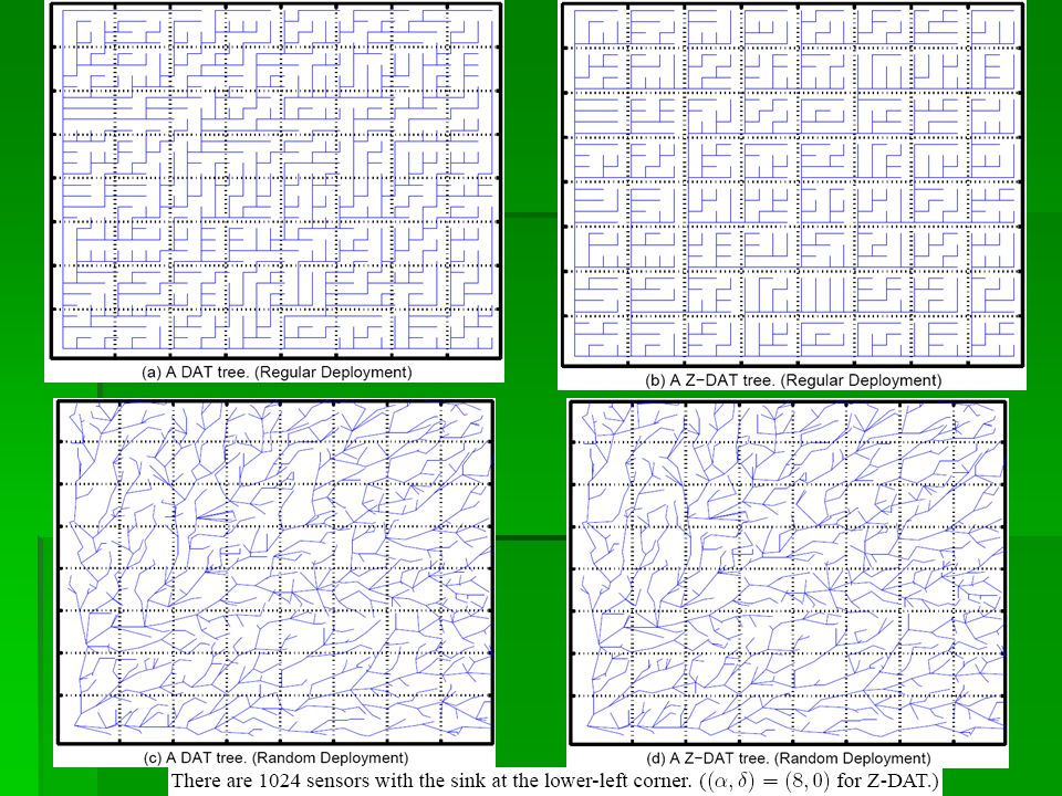
111. Introduction(Cont’)  DAB  the first approach where query messages are not required to be flooded and update messages are not always transmitted to the sink.  drawbacks  a logical tree  Not take the query cost into consideration.  Our tree  first stage : aims at reducing the update cost  Deviation-Avoidance Tree (DAT)  Zone-based Deviation-Avoidance Tree (Z-DAT).  second stage : aims at further reducing the query cost  Query Cost Reduction(QCR) algorithm

112.  Sink  Sensors’ locations are already known  nearest-sensor model  Neighbors  Multiple objects  Event rate(frequency)  the communication range Preliminaries

113. Preliminaries(Cont’)  Graph G = (VG, EG)  VG representing sensors  EG representing links between neighboring sensors  w G (a, b)=sum of event rates from a to b and b to a (weight)

114. Preliminaries(Cont’)  a logical weighted tree T will be constructed from G.

115.  When an object o moves from the sensing range of a to that of b  dep(o, a, b)  arv(o, b, a) Preliminaries(Cont’)

116. Preliminaries(Cont’)  Summary of notations.

117. Tree Construction Algorithms  Algorithm DAT (Deviation-Avoidance Tree)  the avage update cost

118. Tree Construction Algorithms(Algorithm DAT )  three observations  dist T (u, lca(u, v)) minimal value= dist G (u,lca(u, v))  Expect: dist T (u, sink) = dist G (u, sink) for each u  V G  If not: u deviates from its shortest path to the sink  If true for each u  V G : T is a deviation-avoidance tree.  w T (u, v), u  v minimal value is 1  dist T (u,lca(u,v)) + dist T (v,lca(u,v)) can be minimized.  highest-weight-first principle.

120. Tree Construction Algorithms (Algorithm DAT)  Initially, DAT treats each node as a singleton subtree.  Then we will gradually include more links to connect these subtrees together.  In the end, all subtrees will be connected into one tree T.

121. Tree Construction Algorithms (Algorithm DAT)  The DAT growing step  (u, v) will be included into T only if u and v are currently located in different subtrees.  (u, v) will be included into T only if at least one of u and v is currently the root of its temporary subtree and the other is on a shortest path in G from the former node to the sink.

122. Tree Construction Algorithms (Algorithm DAT)

123. Algorithm Z-DAT (Zone- based Deviation- Avoidance Tree)  based on the following locality concept.  Assume that u is v’s parent in T. for any edge (x, y)  E G such that x  Subtree(v) and y  Subtree(v), arrival/departure events between x and y will cause a message to be transmitted on (p(v), v), thus increasing the value of

124. Algorithm Z-DAT (Zone- based Deviation- Avoidance Tree)

125.  The algorithm builds T in an iterative manner based on two parameters,  and , where  is a power of 2 and  is a positive integer.

126. Algorithm QCR (Query Cost Reduction)  QCR is designed to reduce the total update and query cost by adjusting the object tracking tree obtained by DAT/Z- DAT.  Eq 3.

127. Algorithm QCR (Query Cost Reduction)  two observations on Q(T)  because dist T (p(v), sink) is always smaller than dist T (v, sink), Eq. 3 indicates that placing a node as a leaf can save the query cost instead of placing it as a non-leaf.  the second term in Eq. 3 implies that the value of dist T (p(v), sink) should be made as small as possible.

128. Algorithm QCR (Query Cost Reduction)  C(T) - C(T’) = Q(T) - Q(T’) + U(T) - U(T’)

129. Algorithm QCR (Query Cost Reduction)

130. Simulation Results  Update cost environment  a sensing field of size 256 x 256  4096 sensors are deployed in the sensing field  Regularly or randomly deployed  Event rates are generated based on a model similar to the city mobility model C: positive constant d:total number of levels C: positive constant d:total number of levels

131. Simulation Results (Update Cost)

133. Sinks are located at the center of the network. Simulation Results(Update Cost, modify ( ,  )

134. Simulation Results(Query Cost) (C = 1.0)

135. Simulation Results(Total Cost)

136. Conclusion  Made a logical tree reduce the total communication cost incurred by object tracking.  Use DAT and to reduce update cost.  Use Z-DAT to reduce zone communication cost.  Use QCR to improve Z-DAT to reduce query cost.