Download presentation
Presentation is loading. Please wait.

1
Ge277-2010 Stress in the crust Implications for fault mechanics and earthquake physics Motivation Basics of Rock Mechanics Observational constraints on the state of stress in the crust

2
(Bouchon et al., 1997)
")
3
Seismic rupture result from the propagation of a dynamic pulse, possibly as high as 30Mpa Heterogeneities of pre-stress or/and fault strength are needed t explain various aspect of seismic ruptures.

4
Dynamic modeling (Kaneko et et al, in press)
")
6
The complexity (sustained heterogeneities of stress distribution) could be all due to the earthquake process itself, or to inerseismic processes.
 could be all due to the earthquake process itself, or to inerseismic processes.")
8
This can change the conditions along a fault from stable to unstable (= such that displacement occurs) The presence of fluids also induces chemical reactions that may contribute to weaken the fault Pore fluid pressure Water in the pores of rocks produces a pore pressure P f which acts outward, whereas confining pressure acts inward. Hence, fluid pressures can support part of the load across a fault. The pore pressure (eff) thus moves the center of the Mohr circle toward the origin without changing the radius (shear stress keeps the same)
 thus moves the center of the Mohr circle toward the origin without changing the radius (shear stress keeps the same).")
9
= 0.85 N = 0.50+ 0.6 N for N > 200 MPa (Surface roughness becomes less important) ‘base’ coefficient of friction The frictional behavior of rocks can be described by an empirical relation (Byerlee’s law) which, with the exception of some clays, is independent (to first order) of rock type, sliding velocity, surface roughness and temperature (up to 400°C). Frictional strength is related to normal stress (Byerlee, 1978)
.")
10
Static friction measured in lab is generally of the order of 0.6-0.8 (static friction of friction at very slow sliding rate) Dynamic friction (at seismic sliding rates of m/s) can be way lower (<0.1) due to various weakening mechanism. (see Marone 1998, and papers by Toshi Saimamoto’s group on dynamic weakening)
.")
11
Observational constraints on the state of stress in the crust

12
Stress magnitudes derived from the KTB drill hole (Brudy et al, 1997 ) Mohr circles at five different depths compared to the failure lines for a coefficient of friction of 0.6 and 0.8. The Mohr circles are drawn for the following combinations of Sh and SH magnitudes: least Sh value with respective least and greatest SH value, intermediate Sh value with respective least and greatest SH value, and greatest Sh value with respective SH value. (e) Mohr circle for the stress estimation at 7.7 km depth. The circles are drawn for lower and upper bound estimates of the Sh magnitude and the respective lower and upper bounds of the SH magnitude. The effective normal stress is the normal stress minus the hydrostatic pore pressure at the receptive depth. The Mohr circles reach or overcome the failure lines for optimally oriented faults. This means that in the entire investigated depth section, the hypotheses of a frictional equilibrium on preexisting optimally oriented faults with a coefficient between 0.6 and 0.8 is correct.
 Mohr circle for the stress estimation at 7.7 km depth. The circles are drawn for lower and upper bound estimates of the Sh magnitude and the respective lower and upper bounds of the SH magnitude. The effective normal stress is the normal stress minus the hydrostatic pore pressure at the receptive depth. The Mohr circles reach or overcome the failure lines for optimally oriented faults. This means that in the entire investigated depth section, the hypotheses of a frictional equilibrium on preexisting optimally oriented faults with a coefficient between 0.6 and 0.8 is correct..")
13
(Townend and Zoback, 2000 ) Dependence of differential stress on effective mean stress at six locations where deep stress measurements have been made. Dashed lines illustrate relationships predicted using Coulomb frictional-failure theory for various coefficients of friction Evidence for High Deviatoric Stresses consistent with Byerlee Law (hundreds of Mpa at seismogenic depth)
.")
14
It has long been argued that friction on active faults must actually be low, less than about 0.1 : –The absence of heat flow anomaly associated with the SAF (Brune, 1969; Lachenbruch and Sass, 1973) suggests an ambient shear stress<15 Mpa (lithostatic gradient is 27 Mpa/km). Similarly the thermal structure of the Himalaya requires a friction less than 0.1 (Hermann et al, JGR, in Press). NB: Lithostatic gradient is about 27 MPa/km.
. NB: Lithostatic gradient is about 27 MPa/km..")
15
It has long been argued that friction on active faults must be low, less than about 0.1 : –Thrust Sheet mechanics: the thickness-length aspect ration of thrust sheet requires a very low basal friction (for internal deviatoric stress not to exceed crustal rock strength) (Hubert and Ruby, 1959). Analysis based on the critical taper theory generally yield friction less than 0.1 or even lower on decollement (Davis et al, 1983).
..")
16
It has long been argued that friction on active faults must be low, less than about 0.1 : –The maximum horizontal stress near the San Andreas Fault is nearly orhogonal to the fault strike (Zoback et al, 1987).
.")
18
Low effective friction on active faults: –‘Dynamic Weakening’? –High pore pressure? –Inherently weak fault zone? –or something else?

19
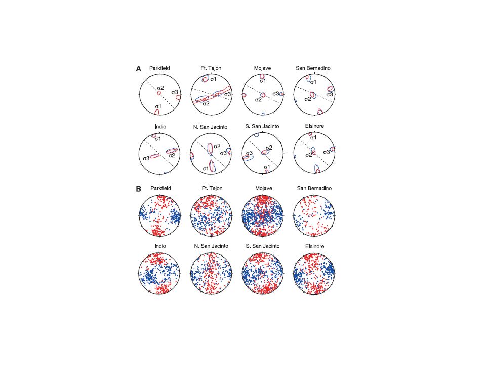
Stress orientation in S. California (Hardebeck and Hauksson, 1999)
")
21
Effect of pore pressure in the fault zone (A) A two-dimensional view perpendicular to the fault. The pore pressure in the surrounding intact rock is hydrostatic, po. The maximum and minimum principal stress axes are in the plane of the cross section, and 1 makes a small angle with the normal to the fault. The fault zone pore pressure, pfz, is elevated and the stress orientations differ from that of the intact rock (B) Mohr circle representation of the same stress states. Open semicircle represents the stress state in the intact rock, and shaded semicircle represents the fault zone. The point common to the two circles is the fault orientation. The Coulomb failure envelopes for pore pressures of po and pfz are shown, and is the angle of internal friction. (C) Sketch of the expected orientation of σ 1 relative to the fault trend versus perpendicular distance from the fault. Shading indicates zone of high fluid pressure. (Rice, 1992; Hardebeck and Hauksson, 1999)
 Mohr circle representation of the same stress states. Open semicircle represents the stress state in the intact rock, and shaded semicircle represents the fault zone. The point common to the two circles is the fault orientation. The Coulomb failure envelopes for pore pressures of po and pfz are shown, and is the angle of internal friction. (C) Sketch of the expected orientation of σ 1 relative to the fault trend versus perpendicular distance from the fault. Shading indicates zone of high fluid pressure. (Rice, 1992; Hardebeck and Hauksson, 1999).")
22
Comparison with the Creeping segment of the San Andreas Fault (Provost and Houston, 2001)
")
23
(Hardebeck&Hauksson, 2001)
")
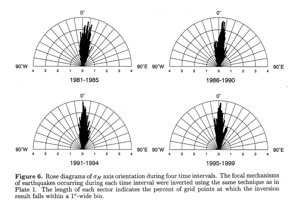
28
(Hardebeck and Hauksson, 2001)
")
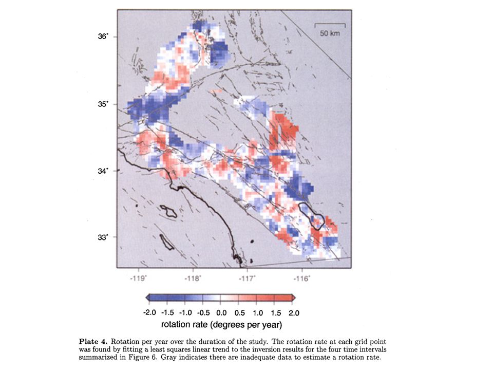
29
Coseismic stress change during the Landers earthquake has induced a rotation of 1 by 15°. (Hardebeck and Hauksson, 2001)
.")
32
Coseismic stress change during the Landers earthquake has induced a rotation of 1 by 15°. This implies that the ratio of the coseismic shear stress change on the fault, to the preexisting deviatoric stress amplitude, is of the order of Δ = 0.65 Given that Δ is estimated to 8 MPa, we infer a =12 Mpa This value is lower by a factor 10 than that predicted from Byerlee’s Law for hydrostatic pore pressure. The fault seems to be ‘weak possibly because of high pore pressure (Hardebeck and Hauksson, 2001)
.")
33
(Hardebeck&Hauksson, 1999)
")
34
Aseismic and Seismic slip If dynamic weakening is responsible for the low shear stress on active faults then the ‘effective’ friction should be higher in creeping zone than where slip is mostly seismic. If high pore pressure is the cause of the low shear stress on active faults then there could be no correlation between slip mode and shear stress.

35
The 2007 Mw 8.0 Pisco Earthquake Paracas Peninsula, Pisco 2007 earthquake, Audin et al., AGU 2007

36
(Sladen et al, JGR, 2010) Coseismic slip model The 2007 Mw 8.0 Pisco Earthquake
 Coseismic slip model The 2007 Mw 8.0 Pisco Earthquake")
37
5/4/2015BSL seminar Post-seismic Displacements following the 2007 Mw 8.0 Pisco Earthquake (Perfettini et al, in press)
")
38
(Perfettini et al, submitted) Afterslip following the 2007 Mw 8.0 Pisco Earthquake - Postseismic displacements reveal two aseismic patches with limited overlap with the coseismic asperities.
 Afterslip following the 2007 Mw 8.0 Pisco Earthquake - Postseismic displacements reveal two aseismic patches with limited overlap with the coseismic asperities.")
39
Static friction Dynamic friction - What are the frictional properties of faults? - How do these properties vary in space and time? - How do they influence individual earthquakes or the long term seismic behavior of a fault? Conceptual framework Some outstanding questions:

40
Conceptual framework Rate&state friction: = * +a ln(V/V * )+b ln( * ) d /dt=1-V /D c ss= * +(a-b) ln(V/V * ) a-b > 0 Rate Strengthening (aseismic slip) a-b < 0 Rate Weakening (seismic slip) At steady state
+b ln( * ) d /dt=1-V /D c ss= * +(a-b) ln(V/V * ) a-b > 0 Rate Strengthening (aseismic slip) a-b < 0 Rate Weakening (seismic slip) At steady state")
41
Interseismic Conceptual framework

42
Coseismic Interseismic Conceptual framework

43
Coseismic Interseismic Postseismic Conceptual framework

44
Fault Frictional Properties (Perfettini and Avouac, 2004) Afterslip governed by rate strenghtening friction should obey: Postseismic
 Afterslip governed by rate strenghtening friction should obey: Postseismic")
45
GE277-AGENDA 2010 January 22: JP January 29: Nina, Sylvain February 5: No Class February 12 : Thomas, Nadaya …

46
Evidence for high deviatoric stress level in the crust [Brudy et al., 1997] JP Dynamic stresses; how earthquakes can help keep the stress level low on faults. [Bouchon et al., 1998]. JP Evidence for low shear stress on active fault. [Hardebeck and Hauksson, 1999; Suppe, 2007]. NADAYA On the influence of fluids; how faulting can keep the crust strong. [Townend and Zoback, 2000]. JEDDY On the influence of fluids, a model of the seismic cycle driven by pore-pressure variations. [Sleep and Blanpied, 1992] THOMAS Inferring fault mechanical properties from geodetic observations [Chang et al., 2009; Perfettini and Avouac, 2004]. ZHONGWEN, NINA? The pb of the trade-off between topology (fault geometry, spatial distribution frictional properties) and intrinsic fault mechanical properties. [Beroza and Mikumo, 1996; Perfettini et al., 2003]. SYLVAIN? Co-seismic slip slip distribution; what does it tell us about fault mechanical properties? [Wesnousky, 2008]. MARION What fraction of fault slip is seismic? [Frohlich and Wetzel, 2007] ANTHONY?
![Evidence for high deviatoric stress level in the crust [Brudy et al., 1997] JP Dynamic stresses; how earthquakes can help keep the stress level low on faults.](http://images.slideplayer.com/13/4142533/slides/slide_46.jpg "[Bouchon et al., 1998]. JP Evidence for low shear stress on active fault. [Hardebeck and Hauksson, 1999; Suppe, 2007]. NADAYA On the influence of fluids; how faulting can keep the crust strong. [Townend and Zoback, 2000]. JEDDY On the influence of fluids, a model of the seismic cycle driven by pore-pressure variations. [Sleep and Blanpied, 1992] THOMAS Inferring fault mechanical properties from geodetic observations [Chang et al., 2009; Perfettini and Avouac, 2004]. ZHONGWEN, NINA. The pb of the trade-off between topology (fault geometry, spatial distribution frictional properties) and intrinsic fault mechanical properties. [Beroza and Mikumo, 1996; Perfettini et al., 2003]. SYLVAIN. Co-seismic slip slip distribution; what does it tell us about fault mechanical properties. [Wesnousky, 2008]. MARION What fraction of fault slip is seismic. [Frohlich and Wetzel, 2007] ANTHONY .")
Similar presentations


 Earthquake Energy Balance>")
 1. Anderson's Theory of Faulting 2. Rheology (mechanical behavior of rocks) - Elastic: Hooke's.>")
 The goal for today is to explore the stress conditions under which rocks fail (e.g., fracture),>")


, Interseismic strain accumulation and anthropogenic motion in metropolitan Los.>")


, Kazuro Hirahara (2), and Mikio Iizuka.>")


