1. Experimental design and analyses of experimental data Lesson 2 Fitting a model to data and estimating its parameters

2. (-2,16) (-1,7) (0,4)(1,6) (2,10) where x 1 = x and x 2 = x 1 2

3. (-2,16) (-1,7) (0,4)(1,6) (2,10) where x 1 = x and x 2 = x 1 2 ε i is the residual for the ith observation

4. The best fit of a model is the one that minimizes the sum of squared deviations between observed and predicted values, i.e.

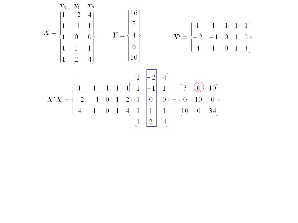
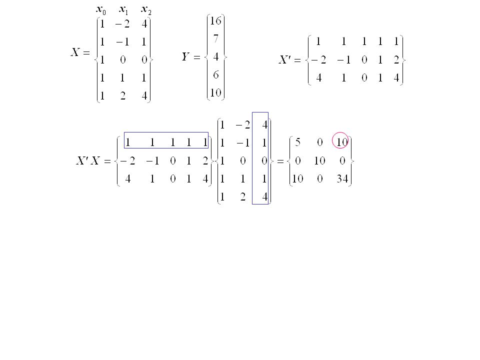
5. How to do the calculations where x 1 = x and x 2 = x 1 2 (x,y) = (-2,16) => y = β 0 (1) + β 1 (-2) + β 2 (4) + ε = 16 (x,y) = (-1,7) => y = β 0 (1) + β 1 (-1) + β 2 (1) + ε = 7 (x,y) = (0,4) => y = β 0 (1) + β 1 (0) + β 2 (0) + ε = 4 (x,y) = (1,6) => y = β 0 (1) + β 1 (1) + β 2 (1) + ε = 6 (x,y) = (2,10) => y = β 0 (1) + β 1 (2) + β 2 (4) + ε = 10 x 0 x 1 x 2 y

6. Transposed X matrix

14. Inverse X’X matrix

15. (X’X) -1 is called the inverse matrix of X’X. It is defined as

17. Variance- covariance matrix

18. Estimation of residual variance (s 2 ) Sum of Squared Errors Degrees of freedom for s 2

19. Variance of estimated parameters Variance-covariance matrix:

20. Covariance of estimated parameters Variance-covariance matrix:

21. Confidence limits for β i

22. Variance of the predicted line Let us assume that we want to predict y for a given value of x The chosen value of x is called a We can now write the equation as

23. Ex. a = -4 Fejl! Skulle have været -1.3

24. V(x+y) = V(x) + V(y) + 2Cov(x,y) V(x-y) = V(x) + V(y) – 2Cov(x,y) V(ax) = a 2 V(x) Cov(ax,by) = abCov(x,y) An alternative way of computation

25. The variance of a new observation of y a = -4 V(y) = (1+15.80)0.829 = 13.92 SE(y) = 3.73 Variance of line Variance of new obs

26. Confidence limits 95% confidence limits for the line: a = -4 95% confidence limits for a single observation:

27. 95% confidence limits

28. How to do it with SAS?

29. DATA eks21; INPUT x y; CARDS; -2 16 -1 7 0 4 1 6 2 10 ; PROC GLM; MODEL y = x x*x/solution ; OUTPUT out= new p= yhat L95M= low_mean U95M = up_mean L95 = low U95 = upper; RUN; PROC PRINT; RUN;

30. Number of observations in data set = 5 General Linear Models Procedure Dependent Variable: Y Source DF Sum of Squares Mean Square F Value Pr > F Model 2 85.54285714 42.77142857 51.62 0.0190 Error 2 1.65714286 0.82857143 Corrected Total 4 87.20000000 R-Square C.V. Root MSE Y Mean 0.980996 10.58441 0.91025899 8.60000000 Source DF Type I SS Mean Square F Value Pr > F X 1 16.90000000 16.90000000 20.40 0.0457 X*X 1 68.64285714 68.64285714 82.84 0.0119 Source DF Type III SS Mean Square F Value Pr > F X 1 16.90000000 16.90000000 20.40 0.0457 X*X 1 68.64285714 68.64285714 82.84 0.0119 T for H0: Pr > |T| Std Error of Parameter Estimate Parameter=0 Estimate INTERCEPT 4.171428571 6.58 0.0224 0.63438867 X -1.300000000 -4.52 0.0457 0.28784917 X*X 2.214285714 9.10 0.0119 0.24327695 OBS X Y YHAT LOW_MEAN UP_MEAN LOW UPPER 1 -2 16 15.6286 11.9426 19.3145 10.2503 21.0068 2 -1 7 7.6857 5.2988 10.0726 3.0991 12.2723 3 0 4 4.1714 1.4419 6.9010 -0.6024 8.9453 4 1 6 5.0857 2.6988 7.4726 0.4991 9.6723 5 2 10 10.4286 6.7426 14.1145 5.0503 15.8068 s2s2 s

31. DATA eks21; INPUT x y; CARDS; -4. -3.5. -3. -2.5. -2 16 -1.5. -1 7 -0.5. 0 4 0.5. 1 6 1.5. 2 10 2.5. 3. 3.5. 4. ; PROC GLM; MODEL y = x x*x/solution ; OUTPUT out= new p= yhat L95M= low_mean U95M = up_mean L95 = low U95 = upper; RUN; PROC PRINT; RUN;

32. OBS X Y YHAT LOW_MEAN UP_MEAN LOW UPPER 1 -4.0. 44.8000 29.2321 60.3679 28.7470 60.8530 2 -3.5. 35.8464 24.1430 47.5499 23.5050 48.1878 3 -3.0. 28.0000 19.6000 36.4000 18.7318 37.2682 4 -2.5. 21.2607 15.5647 26.9568 14.3481 28.1733 5 -2.0 16 15.6286 11.9426 19.3145 10.2503 21.0068 6 -1.5. 11.1036 8.5369 13.6702 6.4210 15.7862 7 -1.0 7 7.6857 5.2988 10.0726 3.0991 12.2723 8 -0.5. 5.3750 2.7660 7.9840 0.6691 10.0809 9 0.0 4 4.1714 1.4419 6.9010 -0.6024 8.9453 10 0.5. 4.0750 1.4660 6.6840 -0.6309 8.7809 11 1.0 6 5.0857 2.6988 7.4726 0.4991 9.6723 12 1.5. 7.2036 4.6369 9.7702 2.5210 11.8862 13 2.0 10 10.4286 6.7426 14.1145 5.0503 15.8068 14 2.5. 14.7607 9.0647 20.4568 7.8481 21.6733 15 3.0. 20.2000 11.8000 28.6000 10.9318 29.4682 16 3.5. 26.7464 15.0430 38.4499 14.4050 39.0878 17 4.0. 34.4000 18.8321 49.9679 18.3470 50.4530

33. A more complex problem Fit a model to these data

34. DATA polynom; INPUT x y; CARDS; 0 8.62 10 -3.99 20 6.80 30 -7.70 40 3.44 50 12.01 60 23.37 70 9.25 80 34.93 90 70.05 100 126.70 ; DATA add; SET polynom; x2 = x**2; x3 = x**3; x4 = x**4; PROC REG; MODEL y = x x2 x3 x4; RUN;

35. The SAS System 08:22 Tuesday, October 29, 2002 1 The REG Procedure Model: MODEL1 Dependent Variable: y Analysis of Variance Sum of Mean Source DF Squares Square F Value Pr > F Model 4 15449 3862.13306 56.59 <.0001 Error 6 409.47543 68.24591 Corrected Total 10 15858 Root MSE 8.26111 R-Square 0.9742 Dependent Mean 25.77091 Adj R-Sq 0.9570 Coeff Var 32.05594 Parameter Estimates Parameter Standard Variable DF Estimate Error t Value Pr > |t| Intercept 1 8.92923 7.90689 1.13 0.3019 x 1 -1.90184 1.21774 -1.56 0.1694 x2 1 0.09562 0.05335 1.79 0.1232 x3 1 -0.00165 0.00082091 -2.01 0.0917 x4 1 0.00000999 0.00000407 2.45 0.0495 A fourth order polynomium

36. The SAS System 08:22 Tuesday, October 29, 2002 2 The REG Procedure Model: MODEL1 Dependent Variable: y Analysis of Variance Sum of Mean Source DF Squares Square F Value Pr > F Model 3 15037 5012.44667 42.75 <.0001 Error 7 820.66769 117.23824 Corrected Total 10 15858 Root MSE 10.82766 R-Square 0.9482 Dependent Mean 25.77091 Adj R-Sq 0.9261 Coeff Var 42.01505 Parameter Estimates Parameter Standard Variable DF Estimate Error t Value Pr > |t| Intercept 1 1.73490 9.62511 0.18 0.8621 x 1 0.59619 0.87649 0.68 0.5182 x2 1 -0.02928 0.02099 -1.39 0.2057 x3 1 0.00035168 0.00013776 2.55 0.0379 A third order polynomium

37. The SAS System 08:22 Tuesday, October 29, 2002 3 The REG Procedure Model: MODEL1 Dependent Variable: y Analysis of Variance Sum of Mean Source DF Squares Square F Value Pr > F Model 2 14273 7136.65872 36.03 <.0001 Error 8 1584.69025 198.08628 Corrected Total 10 15858 Root MSE 14.07431 R-Square 0.9001 Dependent Mean 25.77091 Adj R-Sq 0.8751 Coeff Var 54.61318 Parameter Estimates Parameter Standard Variable DF Estimate Error t Value Pr > |t| Intercept 1 14.39524 10.72255 1.34 0.2163 x 1 -1.41540 0.49888 -2.84 0.0219 x2 1 0.02347 0.00480 4.88 0.0012 A second order polynomium

38. The SAS System 08:22 Tuesday, October 29, 2002 4 The REG Procedure Model: MODEL1 Dependent Variable: y Analysis of Variance Sum of Mean Source DF Squares Square F Value Pr > F Model 1 9547.03680 9547.03680 13.61 0.0050 Error 9 6310.97089 701.21899 Corrected Total 10 15858 Root MSE 26.48054 R-Square 0.6020 Dependent Mean 25.77091 Adj R-Sq 0.5578 Coeff Var 102.75361 Parameter Estimates Parameter Standard Variable DF Estimate Error t Value Pr > |t| Intercept 1 -20.81000 14.93704 -1.39 0.1970 x 1 0.93162 0.25248 3.69 0.0050 A first order polynomium (a straight line)

39. True relationship: y = 5 + 0.1x – 0.02x 2 + 0.0003x 3 + ε ε is normally distributed with 0 mean and σ = 10 Estimated relationship: y = 14.395 – 1.415x + 0.0235x 2 s = 14.07 Estimated relationship: y = -20.81 + 0.932x s = 26.48 This is a better fit than this

40. Matrix Notation Of particular interest to us is the fact that not even in regression analysis was much use made of matrix algebra. In fact one of us, as a statistics graduate student at Cambridge University in the early 1950s, had lectures on multiple regression that were couched in scalar notation! This absence of matrices and vectors is surely surprising when one thinks of A.C. Aitken. His two books, Matrices and Determinants and Statistical Mathematics were both first published in 1939, had fourth and fifth editions, respectively, in 1947 and 1948, and are still in print. Yet, very surprisingly, the latter makes no use of matrices and vectors which are so thoroughly dealt with in the former. There were exceptions, of course, as have already been noted, such as Kempthorne (1952) and his co-workers, e.g. Wilk and Kempthorne (1955, 1956) – and others, too. Even with matrix expressions available, arithmetic was a real problem. A regression analysis in the New Zealand Department of Agriculture in the mid-1950s involved 40 regressors. Using electromechanical calculators, two calculators (people) using row echelon methods needed six weeks to invert the 40 x 40 matrix. One person could do a row, then the other checked it (to a maximum capacity of 8 to 10 digits, hoping for 4- or 5-digit accuracy in the final result). That person did the next row and passed it to the first person for checking; and so on. This was the impasse: matrix algebra was appropriate and not really difficult. But the arithmetic stemming therefrom could be a nightmare. (From Linear Models 1945-1995 by Shayle R. Searle and Charles E. McCulloch in Advances in Biometry (eds. Peter Armitage and Herbert A. David), John Wiley & Sons, 1996)