Download presentation
Presentation is loading. Please wait.

1
CHAPTER V CONTROL SYSTEMS
Process Control CHAPTER V CONTROL SYSTEMS

3
For the mathematical analysis of control systems it’s possible to consider the controller as a simple computer. For example, a proportional controller may be thought of as a device which receives the error signal and puts out a signal proportional to it. Similarly, the final control element may be considered as a device which produces corrective action (related with output signal of the controller) on the process. In industry final control elements are operated electronically in most of the cases. However, here a pneumatic (needs air to operate) valve is chosen in order to understand the details.
 on the process. In industry final control elements are operated electronically in most of the cases. However, here a pneumatic (needs air to operate) valve is chosen in order to understand the details..")
4
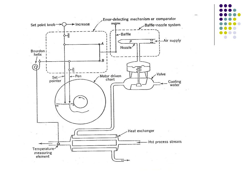
In the system, there exists a heat exchanger which is used to cool down the hot stream. The temperature of the outlet stream is continuously measured and changing the flow rate of the cooling water temperature is controlled. If temperature rises the pressure in mercury filled bulb (which senses temperature) increases and pressure in the Bourdon helix increases causing it to unwind. The motion of the helix moves the pen across the chart and moves the baffle towards the nozzle. This baffle motion is made proportional to the pen motion by proper linkage.
 increases and pressure in the Bourdon helix increases causing it to unwind. The motion of the helix moves the pen across the chart and moves the baffle towards the nozzle. This baffle motion is made proportional to the pen motion by proper linkage.")
5
The baffle motion results in a proportional increase in pressure in nozzle and valve top which result an increase in cooling water flow. As the baffle is moved toward the nozzle, the pressure P in the nozzle increases because the area for air discharge is reduced. The nozzle pressure becomes equal to the supply pressure when the nozzle is closed by the baffle and the system is so designed that the nozzle pressure falls linearly as the baffle to nozzle distance is increased.

6
With the increase in pressure the plug moves downward and supplies the flow of cooling water through the valve. In general, the flow rate of the fluid through the valve depends upon the upstream and downstream fluid pressures and the size of the opening through the valve. In this system, we assume that at steady state, the flow is proportional to the valve top pneumatic pressure. A valve with this relation is called a linear valve.

7
Transfer function for a control valve
From the previous experimental studies conducted on pneumatic valves it has been found that the relationship between flow rate and valve top pressure for a linear valve can be represented by a first-order transfer function. In many practical systems, the time constant of the valve is very small compared with the time constants of other components of the control system. Therefore, the transfer function of the valve can be approximated by a constant.

8
TRANSFER FUNCTIONS FOR CONTROLLERS
The transfer functions in the following part are developed for pneumatic controllers. For electronic controllers, the same equations are applicable by changing (P) with suitable representation of the signal. Proportional control (P Control) The proportional controller produces an output signal which is proportional to the error ε. Where; p: output pressure signal from controller Kc: gain or sensitivity (adjustable) ε: error, (ε = set point-measured variable) ps usually adjustable to obtain the required output
 with suitable representation of the signal. Proportional control (P Control) The proportional controller produces an output signal which is proportional to the error ε. Where; p: output pressure signal from controller. Kc: gain or sensitivity (adjustable) ε: error, (ε = set point-measured variable) ps usually adjustable to obtain the required output.")
9
Kc : controller gain, proportionality constant
The controller gain can be adjusted to make the controller output changes as sensitive as desired to deviations in error. The sign can be chosen to make the controller output increase (or decrease) as the error signal increases. It’s usually adjusted after the controller has been installed.
 as the error signal increases. It’s usually adjusted after the controller has been installed.")
10
In order to obtain transfer functions deviation variables should be introduced.
P=p-ps ε is already a deviation variable (at t=0, εs =0) therefore,
 therefore,")
11
Disadvantage; a steady-state error (offset) occurs after a set-point change or a sustained disturbance. This can be eliminated by manually resetting either the set-point or steady-state value after an offset occurs. However, this approach is inconvenient because; to have the change an operator intervention is required new value must usually be found by trial and error. Advantage; for control applications where offsets can be tolerated, proportional control is attractive because of its simplicity.

12
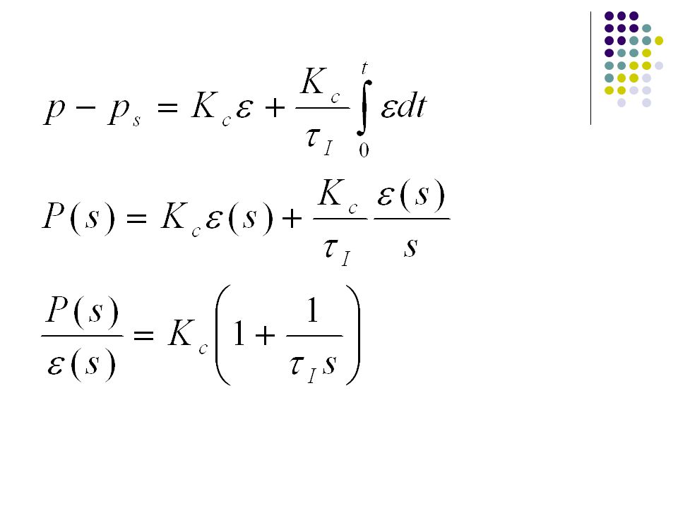
ii. Proportional-integral control (PI Control)
This mode of control is described by the relationship, where, Kc: gain τI: integral time ps: constant set-up this term is proportional to the integral of the error. The Kc and τI values are adjustable.

13
Advantage: In integral control offset will be eliminated
Advantage: In integral control offset will be eliminated. Thus, when integral control is used “p” automatically changes until it attains the value required to make the steady-state error zero. Although elimination of offset is usually an important control objective, integral control is not used by itself because little control action takes place until the error signal has persistent for some time. In contrast, proportional control action takes immediate corrective action as soon as an error is detected. Therefore, integral control action is normally used in conjunction with proportional control as the proportional-integral (PI) controller. Disadvantage: Integral control action tends to produce oscillatory responses of the controlled variable which affects stability.
 controller. Disadvantage: Integral control action tends to produce oscillatory responses of the controlled variable which affects stability.")
15
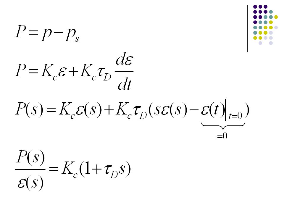
iii. Proportional-derivative control (PD Control)
This mode of control is described by the relationship: where, Kc: gain τD: derivative time Ps: constant in this term correction is proportional to the derivative of the error. Derivative control action tends to improve the dynamic response of the controlled variable by decreasing the process settling time (i.e., the time it takes the process to reach steady-state). In application , PD control algorithm is physically undesirable since it can not be implemented exactly using analog or digital components.
. In application , PD control algorithm is physically undesirable since it can not be implemented exactly using analog or digital components.")
17
iv . Proportional-derivative-integral control
This mode of control is a combination of the previous models and is given by; where, KC, τD and τI are adjustable. The transfer function for this mode of control is given as

18
Example for proportional-integral control
Example for proportional-integral control. Where, unit step change in error i.e., ε(t)=1 Example for proportional-derivative control. Where, ε(t)=A.t
=1. Example for proportional-derivative control. Where, ε(t)=A.t.")
19
no control Deviation variable proportional control proportional-integral control Time (min) proportional-integral-derivative control

20
If disturbance occurs the value of the controlled variable starts to rise. Without control this variable continues to rise to a new steady-state value. With proportional action only, the control system can stop the rise of the controlled variable and ultimately bring it to rest at a new steady-state value. The difference between this new steady-state value and the original value is called “offset”.

21
The addition of integral action eliminates the offset, the controlled variable ultimately returns to the original value. The disadvantage of this action is a more oscillatory behavior. With the addition of derivative action the response will be improved. The rise of the controlled variable is stopped more quickly and its returned rapidly to the original value with little or no oscillation.

22
First-order Systems τ: time constant Kp: steady state gain

23
They have capacity to store material, energy or momentum.
There exists a resistance with the flow of mass, energy or momentum associated with pumps, valves, weirs and pipes. A first order system is self-regulating : (time constant) is a measure of the time necessary for the process to adjust to a change in input. Time elapsed y(t) as % of ultimate value
 is a measure of the time necessary for the process to adjust to a change in input. Time elapsed. y(t) as % of ultimate value.")
24
to have the same change in the output:
At steady state to have the same change in the output: a small change in input is required if Kp is large (very sensitive) a large change in input is required if Kp is small.
 a large change in input is required if Kp is small.")
25
Second-order systems Multicapacity processes (i.e., two or more first order systems) Inherently second order systems (having inertia) A processing system with its controller

26
Example: Obtaining the transfer function for a first order system with a capacity for mass storage.
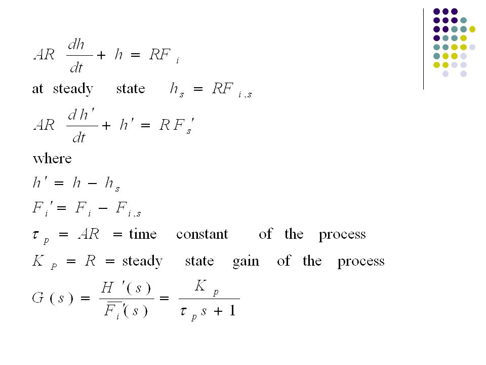
Consider the tank shown in figure. The volumetric flow in is Fi and the outlet volumetric flow rate is Fo. In the outlet stream there is a resistance to flow, such as a pipe, valve or weir. Fi Fi h h Fo R Fo

27
Assume that the effluent flow rate Fo is related linearly to the hydrostatic pressure of the liquid level h, through the resistance R: The total mass balance gives;

29
The cross-sectional area of the tank A is a measure of its capacitance to store mass. Thus the larger the value of A, the larger the storage capacity of the tank. Since time constant is defined as AR, we can say that, (time constant)=(storage capacitance) x (resistance to flow)
=(storage capacitance) x (resistance to flow)")
Similar presentations


 relates one input and one output: The following terminology.>")

 relates one input and one output: The following terminology.>")


