1. Spectral functions in NRG Rok Žitko Institute Jožef Stefan Ljubljana, Slovenia

2. Green's functions - review Following T. Pruschke: Vielteilchentheorie des Festkorpers + if A and B are fermionic operators - if A and B are bosonic operators NOTE: ħ=1 Also known as the retarded Green's function.

3. Laplace transformation: Impurity Green's function (for SIAM): Inverse Laplace transformation:

4. Equation of motion Example 1:

5. Example 2:

6. Example 3: resonant-level model Here we have set  =0. Actually, this convention is followed in the NRG, too.

7. Hybridization function: fully describes the effect of the conduction band on the impurity

8. Spectral decomposition  =+1 if A and B are fermionic, otherwise  =-1.  spectral representation spectral function

10. Lehmann representation

11. Fluctuation-dissipation theorem Useful for testing the results of spectral-function calculations! Caveat: G"(  ) may have a delta peak at  =0, which NRG will not capture.

12. Dynamic quantities: Spectral density Spectral density/function: Describes single-particle excitations: at which energies it is possible to add an electron (ω>0) or a hole (ω<0).

13. Traditional way: at NRG step N we take excitation energies in the interval [a  N : a  1/2  N ] or [a  N : a   N ], where a is a number of order 1. This defines the value of the spectral function in this same interval.

14. Patching

15. p p  1/2 pp p: patching parameter (in units of energy scale at N+1-th iteration)

16. Broadening: traditional log-Gaussian smooth=old

17. Broadening: modified log-Gaussian smooth=wvd for x<  0, 1 otherwise.

18. Broadening: modified log-Gaussian smooth=new Produces smoother spectral functions at finite temperatures (less artifacts at  =T).

19. Other kernels smooth=newsc smooth=lorentz For problems with a superconducting gap (below  ). If a kernel with constant width is required (rarely!).

20. Log-Gaussian broadening 1) Features at  =02) Features at  ≠0

22. Equations of motion for SIAM:

23. Self-energy trick

25. Non-orthodox approach: analytic continuation usng Padé approximants We want to reconstruct G(z) on the real axis. We do that by fitting a rational function to G(z) on the imaginary axis (the Matsubara points). This works better than expected. (This is an ill-posed numerical problem. Arbitrary-precision numerics is required.) Ž. Osolin, R. Žitko, arXiv:1302.3334arXiv:1302.3334

29. Kramers-Kronig transformation

31. Inverse-square-root asymptotic behavior

32. Doniach, Šunjić 1970 J. Phys. C: Solid State Phys. 3 285 Inverse square root behavior also found using the quantum Monte Carlo (QMC) approach: Silver, Gubernatis, Sivia, Jarrell, Phys. Rev. Lett. 65 496 (1990) Anderson orthogonality catastrophe physics

34. Arguments: Kondo model features characteristic logarithmic behavior, i.e., as a function of T, all quantities are of the form [ln(T/T K )] -n. Better fit to the NRG data than the Doniach-Šunjić form. (No constant term has to be added, either.)

35. Osolin, Žitko, 2013

36. Comparison with experiment?

37. Experiment, Ti (S=1/2) on CuN/Cu(100) surface A. F. Otte et al., Nature Physics 4, 847 (2008) NRG calculation Excellent agreement (apart from asymmetry, presumably due to some background processes)

38. 1/  tail Kondo resonance is not a simple Lorentzian, it has inverse-square-root tails!

39. Fano-like interference process between resonant and background scattering:

40. RŽ, Phys. Rev. B 84, 195116 (2011)

41. Density-matrix NRG Problem: Higher-energy parts of the spectra calculated without knowing the true ground state of the system Solution: 1) Compute the density matrix at the temperature of interest. It contains full information about the ground state. 2) Evaluate the spectral function in an additional NRG run using the reduced density matrix instead of the simple Boltzmann weights.

42. W. Hofstetter, PRL 2000

43. DMNRG for non-Abelian symmetries: Zitko, Bonca, PRB 2006

44. Spectral function computed as: W. Hofstetter, PRL 2000

45. Construction of the complete basis set

46. Completeness relation: Complete-Fock-space NRG: Anders, Schiller, PRL 2005, PRB 2006

47. Peters, Pruschke, Anders, PRB 2006

48. Full-density-matrix NRG: Weichselbam, von Dellt, PRL 2007 Costi, Zlatić, PRB 2010

49. CFS vs. FDM vs. DMNRG CFS and FDM equivalent at T=0 FDM recommended at T>0 CFS and FDM are slower than DMNRG (all states need to be determined, more complex expressions for spectral functions) No patching, thus no arbitrary parameter as in DMNRG

50. Rok Žitko, PRB 84, 085142 (2011) Error bars in NRG?

51. Average + confidence region!

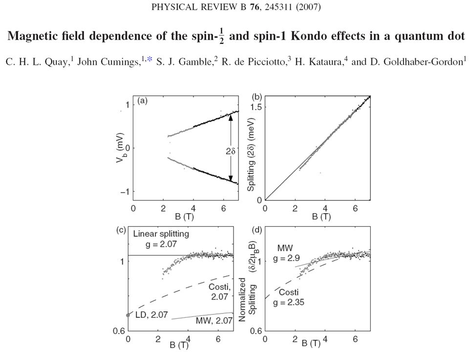
52. Effect of the magnetic field: resonance splitting A. F. Otte et al., Nature Physics 4, 847 (2008) Ti atom S=1/2

53. Numerical renormalization group (NRG) calculation

54. Bethe Ansatz calculation using spinon density of states

55. Exact result for B→0: Δ=(2/3)g  B B Suggestion that for large B, Δ is larger than g  B B.

56. gives 2/3 for R=2, in agreement with Logan et al. (Factor 2 due to different convention.) Also find that Δ > 1g  B B, but they note that this might be non-universal behavior due to charge fluctuations in the Anderson model (as opposed to the Kondo model).

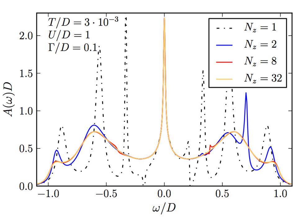
58. Interrelated problems: systematic discretization errors and spectral broadening  determines how  peaks are smoothed out!

59. Pessimistic error bars Rok Žitko, PRB 84, 085142 (2011)

60. Optimistic error bars The correct result is obtained in the  →0 limit!

61. NRG Agreement within error bars!

62. Experimental results for Ti adatoms: F. Otte et al., Nature Physics 4, 847 (2008) NRG calculation R. Ž., submitted B=7 T

63. Kondo model