Download presentation
Presentation is loading. Please wait.

1
MULTIDIMENSIONAL POVERTY AND DEPRIVATION to be presented by Jacques Silber Department of Economics Bar-Ilan University – Israel at the Fourth Winter School on Inequality and Social Welfare Theory (IT4)
")
2
INTRODUCTION I would like to start this lecture by citing a very known social philosopher of the nineteenth century, Alexis de Tocqueville. Alexis de Tocqueville who is known for his famous “Democracy in America” and eventually also for his “The Old Regime and the Revolution” wrote also a monography entitled “Memoir on Pauperism”. I must say that until I looked at a book by the French sociologist Serge Paugam entitled “The Elementary Forms of Poverty” I was totally unaware of Tocqueville´s Memoir. Tocqueville was born in 1805 and died in 1859. His Memoir on Pauperism was written in 1835, immediately after he completed the first volume of Democracy in America. In the first part of this Memoir Tocqueville stressed that there was a difference between individuals who are “poor” and those who are “indigents”. The latter are people who can be clearly distinguished within a population (hence the modern concept of “social exclusion”). In the first part of his Memoir Tocqueville makes an interesting comparison between England on one hand and Spain and Portugal on the other.
. In the first part of his Memoir Tocqueville makes an interesting comparison between England on one hand and Spain and Portugal on the other..")
3
“Cross the English countryside and you will think yourself transported into the Eden of modern civilization….There is a pervasive concern for well-being and leisure, an impression of universal prosperity which seems part of every air you breathe… Now look more closely at the villages: examine the parish registers and you will discover with indescribable astonishment that one-sixth of the inhabitants of this flourishing kingdom live at the expense of public charity” Now, if you turn to Spain, or even more to Portugal, you will be struck by a very different sight. You will see at every step an ignorant and coarse population; ill-fed, ill-clothed, living in the midst of a half- uncultivated countryside and in miserable dwellings. In Portugal, however, the number of indigents is insignificant….” This is a description of three countries in the middle of the nineteenth century, even before. But it seems to me that this distinction between the “poor” and the “indigents” remains a valid one today. The only difference is that today specialists use other words, making, for example, a distinction between the “income poor” and the “socially excluded”.

4
Part II of Tocqueville´s Memoir is more policy-oriented, condemning the Poor Laws. But the distinction he made between the “poor” and the “indigents” remains of central importance today, although it tends to be hidden behind the labels of unidimensional versus multidimensional poverty.

5
Measuring Poverty: Taking a Multidimensional Approach. The goal of my lecture is to attempt - to review the main problems that have to be faced when taking a multidimensional approach to poverty -to give a survey of the solutions that have hitherto been proposed to solve these problems although I will emphasize some solutions more than others, in order not to duplicate Jean-Yves Duclos’ lecture tomorrow. -I will thus leave it to Jean-Yves to talk about the axiomatic as well as the ordinal approach to multidimensional poverty measurement.

6
Outline of Talk I) The Cardinal Approach to Multidimensional Poverty Measurement: A) Important Issues in Multidimensional Poverty Analysis: 1) The Choice of the Poverty Dimensions 2) The “Fuzzy Aspect” of Poverty 3) The “Vertical Vagueness” of Poverty 4) The “Temporal Vagueness” of Poverty:
 The Cardinal Approach to Multidimensional Poverty Measurement: A) Important Issues in Multidimensional Poverty Analysis: 1) The Choice of the Poverty Dimensions 2) The Fuzzy Aspect of Poverty 3) The Vertical Vagueness of Poverty 4) The Temporal Vagueness of Poverty:")
7
B) The Case where Dimensions are aggregated immediately: 1) Approaches using traditional multivariate analysis 2) The so-called Rasch model 3) Efficiency Analysis and Multidimensional Poverty 4) Information Theory 5) The concept of order of acquisition of durable goods C) Determining first poverty lines for each dimension, then aggregating the dimensions and finally aggregating the individual observations 1) The axiomatic approach to multidimensional poverty measurement 2) Information theory 3) The Subjective approach to multidimensional poverty measurement 4) Alkire and Foster’s (2007) recent proposal D) Determining first poverty lines for each dimension, then aggregating the individual observations and finally aggregating the dimensions: The Fuzzy Approach
 The Case where Dimensions are aggregated immediately: 1) Approaches using traditional multivariate analysis 2) The so-called Rasch model 3) Efficiency Analysis and Multidimensional Poverty 4) Information Theory 5) The concept of order of acquisition of durable goods C) Determining first poverty lines for each dimension, then aggregating the dimensions and finally aggregating the individual observations 1) The axiomatic approach to multidimensional poverty measurement 2) Information theory 3) The Subjective approach to multidimensional poverty measurement 4) Alkire and Foster’s (2007) recent proposal D) Determining first poverty lines for each dimension, then aggregating the individual observations and finally aggregating the dimensions: The Fuzzy Approach")
8
E) Does the selection of a specific approach make a difference? II) The Qualitative Approach and Learning from other Social Sciences: Anthropology Participatory Approaches CONCLUDING COMMENTS
 The Qualitative Approach and Learning from other Social Sciences: Anthropology Participatory Approaches CONCLUDING COMMENTS.")
9
I) The Cardinal Approach to Multidimensional Poverty Measurement: In what follows a distinction will be made first between (1)approaches that lead to the derivation of an aggregate indicator on the basis of which a poverty threshold (line) will be determined and traditional measures of uni-dimensional poverty will be derived (2) truly multidimensional approaches where a poverty threshold is determined for each dimension and which lead to the definition of multidimensional indices of poverty. But in the case of (2) two possibilities again arise: a)Aggregate first the dimensions and then the individuals b)Aggregate first the individuals and then the dimensions The following graph attempts to describe the various ways of deriving a multidimensional poverty index.
 two possibilities again arise: a)Aggregate first the dimensions and then the individuals b)Aggregate first the individuals and then the dimensions The following graph attempts to describe the various ways of deriving a multidimensional poverty index..")
11
Before reviewing these approaches I would like to mention additional issues that are somehow specific to the multidimensional case. A) On Some Important Issues in Multidimensional Poverty Analysis: 1)The Choice of the Poverty Dimensions: Several questions have to be asked: a) Which DIMENSIONS are relevant? b) Should more than one INDICATOR per dimension be used, and if so which ones? c) Which kind of INTERACTION BETWEEN DIMENSIONS should one assume? Are Dimensions SUBSTITUTES or COMPLEMENTS? d) How to deal with INTERACTIONS BETWEEN INDICATORS representing a given dimension?
 On Some Important Issues in Multidimensional Poverty Analysis: 1)The Choice of the Poverty Dimensions: Several questions have to be asked: a) Which DIMENSIONS are relevant. b) Should more than one INDICATOR per dimension be used, and if so which ones. c) Which kind of INTERACTION BETWEEN DIMENSIONS should one assume. Are Dimensions SUBSTITUTES or COMPLEMENTS. d) How to deal with INTERACTIONS BETWEEN INDICATORS representing a given dimension .")
12
The issue of the interaction between the dimensions will be covered by Jean-Yves Duclos. Just a few words on the selection of dimensions: Sabina Alkire (2008) listed five possible ways of selecting dimensions: -Decide in function of the availability of data or because of an authoritative convention -Make implicit or explicit assumptions about what people value -Follow “Public Consensus” (e.g. list of Millenium Development Goals or MDG´s) -Rely on deliberative participatory processes -Accept empirical evidence concerning people´s values
 listed five possible ways of selecting dimensions: -Decide in function of the availability of data or because of an authoritative convention -Make implicit or explicit assumptions about what people value -Follow Public Consensus (e.g. list of Millenium Development Goals or MDG´s) -Rely on deliberative participatory processes -Accept empirical evidence concerning people´s values.")
13
An Illustration: Ramos and Silber (2005) This paper attempted to translate empirically some of the approaches mentioned by Alkire (2002) in her paper on The Dimensions of Human Development. One of the approaches she mentioned is that of Allardt whose ideas were presented in his paper on “Having, Loving, Being: An Alternative to the Swedish Model of Welfare Research” (in Nussbaum and Sen, The Quality of Life).
..")
14
Thus, using the British Household Panel Survey, we took into account the following dimensions: A) HAVING: 1)Economic resources 2)Housing 3)Employment 4)Working Conditions 5)Health 6)Education B) LOVING: Satisfaction with social life (family, friends,…) C) BEING: 1)Self-Determination (ability making decisions,…) 2)Political Activities 3)Leisure Time Activities 4)Opportunities to Enjoy Nature 5)Meaningful Work (Satisfaction with work,…) Clearly selecting dimensions is not a simple issue and Clark and Qizilbash (2005) have labelled this problem the “horizontal vagueness” of poverty.
 HAVING: 1)Economic resources 2)Housing 3)Employment 4)Working Conditions 5)Health 6)Education B) LOVING: Satisfaction with social life (family, friends,…) C) BEING: 1)Self-Determination (ability making decisions,…) 2)Political Activities 3)Leisure Time Activities 4)Opportunities to Enjoy Nature 5)Meaningful Work (Satisfaction with work,…) Clearly selecting dimensions is not a simple issue and Clark and Qizilbash (2005) have labelled this problem the horizontal vagueness of poverty.")
15
2) The “Fuzzy Aspect” of Poverty: The problem here is that determining a clear threshold making a difference between those who are poor and those who are not is not an easy task. A reasonable solution may be found, say, in the “nutrition dimension” (e.g. minimum number of calories needed as a function of age, location, …). The issue is more complex when dealing with, for example, a “shelter” or an income dimension. We will come back to this issue when describing the so-called Fuzzy Appproach to Multidimensional poverty.
. The issue is more complex when dealing with, for example, a shelter or an income dimension. We will come back to this issue when describing the so-called Fuzzy Appproach to Multidimensional poverty..")
16
3) The “Vertical Vagueness” of Poverty: Clark and Qizilbash (2005) have used the expression “vertical vagueness” to emphasize that deciding which individual (household) is poor is not an easy task in a multidimensional framework. Should be called “poor” only those individuals (households) who are poor in all dimensions or is it enough to be poor in one dimension to be called “poor”? Jean-Yves Duclos will probably discuss this choice between an approach focussing on the concept of “union” and another one stressing that of “intersection”.
 who are poor in all dimensions or is it enough to be poor in one dimension to be called poor . Jean-Yves Duclos will probably discuss this choice between an approach focussing on the concept of union and another one stressing that of intersection ..")
17
4) The “temporal vagueness” of poverty: Finally Clark and Qizilbash have also introduced the concept of “temporal vagueness” which refers to the unit of time one should select when analyzing poverty. The importance of time may in fact be considered from different angles. -the contrast between Chronic and Transitory Poverty -the idea of Vulnerability

18
A) On Chronic versus Transitory Poverty: A citation from Hulme and McKay (2008): “For many people poverty is not a transitory experience or a seasonal problem: it is a situation from which escape is very difficult, most emphatically illustrated by deprivation which is transmitted from one generation to the next”. As stressed by these authors a similar distinction was made in eighteenth century France when a distinction was made between the pauvres and the indigents. “The former experienced seasonal poverty when crops failed or demand for casual agricultural labour was low. The latter were permanently poor because of ill health (physical and mental), accident, age, alcoholism or other forms of ‘vice’ “.
, accident, age, alcoholism or other forms of ‘vice’ ..")
19
Hulme and Shepherd (2003) identify four main ways in which people may experience chronic poverty: -those who experience poverty for a long time (five years, more?). -those who experience poverty throughout their entire lives (life course poverty) -the transfer of poverty from parents to children (inter-generational poverty) -those who experience a premature death that was easily preventable.
 -the transfer of poverty from parents to children (inter-generational poverty) -those who experience a premature death that was easily preventable..")
20
This is why, following work by Carter and Barrett (2006), these authors recommend using an asset approach to poverty measurement and make eventually a distinction between structural and stochastic poverty. Consider a transitorily poor household that is poor in the first period but above the poverty line in the second period. This may reflect structural change, because for example the household has been able to accumulate assets over this period. Alternatively it may reflect stochastic factors: the fact that the household was poor in one of the two periods may just be the consequence of bad luck in that period. This is why the question to be asked is whether on average that level of assets is sufficient to put a household above the poverty line, hence the idea of an asset poverty line.

21
The goal is to be able to distinguish among the income poor (as well as non-poor) between those for whom this situation appears to be temporary because they have (do not have) a sufficiently high level of assets, and those for whom this seems to be permanent. Carter and Barrett (2006) think thus in terms of a dynamic asset threshold which is somehow the level above which households will save and accumulate assets (keeping them above the poverty line), and below which they will reduce their asset holdings and find themselves in a situation of long term poverty (poverty trap).
 think thus in terms of a dynamic asset threshold which is somehow the level above which households will save and accumulate assets (keeping them above the poverty line), and below which they will reduce their asset holdings and find themselves in a situation of long term poverty (poverty trap)..")
22
B) The concept of “vulnerability”: Calvo and Dercon (2008) stress the importance of the ex-ante consequences of the possibility of future hardship. For them vulnerability is viewed as the magnitude of the threat of poverty, measured ex-ante, before the veil of uncertainty has been lifted. There is a nice citation from Voices of the Poor (2000) which can be found also in Calvo (2008): “Security is peace of mind and the possibility to sleep relaxed” (a woman from El Gawaber, Egypt). Calvo and Dercon give the following illustration, borrowed from Sen (1981) who discusses the famine in Sahel.: “Compared with the farmer or the pastoralist who lives on what he grows and is thus vulnerable only to variations of his own output (arising from climatic considerations or other influences), the grower of cash crops, or the pastoralist heavily dependent on selling animal products, is vulnerable both to output fluctuations and to shifts in marketability of commodities and in exchange rates.…[Thus] while commercialization may have opened up new economic opportunities, it has also tended to increase the vulnerability of the Sahel population”.
 which can be found also in Calvo (2008): Security is peace of mind and the possibility to sleep relaxed (a woman from El Gawaber, Egypt). Calvo and Dercon give the following illustration, borrowed from Sen (1981) who discusses the famine in Sahel.: Compared with the farmer or the pastoralist who lives on what he grows and is thus vulnerable only to variations of his own output (arising from climatic considerations or other influences), the grower of cash crops, or the pastoralist heavily dependent on selling animal products, is vulnerable both to output fluctuations and to shifts in marketability of commodities and in exchange rates.…[Thus] while commercialization may have opened up new economic opportunities, it has also tended to increase the vulnerability of the Sahel population ..")
23
To be more explicit, vulnerability has to do with “the probability of outcomes failing to reach some minimal standard and on the uncertainty about how far below that threshold the outcome may finally turn out to be. States of the world where outcomes are above the poverty threshold are paid no attention, so that vulnerability is not lessened by simultaneous ex ante possibilities of very high outcomes” (Calvo, 2008).
..")
24
B) The Case where Dimensions are aggregated immediately: Many techniques of aggregation have been proposed. We cannot review all of them (for more details, see, Kakwani and Silber, 2008) but will at least mention some of them. 1)Approaches using traditional multivariate analysis: These approaches are generally based on the idea of latent variable. Here we should mention the following techniques: -Principal Components Analysis (PCA) -Factor Analysis (FA) -MIMIC models -Structural Equation models -Cluster Analysis -Multiple Correspondance Analysis (MCA)
 but will at least mention some of them. 1)Approaches using traditional multivariate analysis: These approaches are generally based on the idea of latent variable. Here we should mention the following techniques: -Principal Components Analysis (PCA) -Factor Analysis (FA) -MIMIC models -Structural Equation models -Cluster Analysis -Multiple Correspondance Analysis (MCA).")
25
a)Principle Components Analysis: Principal Components Analysis (PCA) seeks linear combinations of the observed indicators in such a way as to reproduce the original variance as closely as possible. It is thus an “aggregating technique” but lacks an underlying explanatory model which factor analysis offers.

26
b) Factor Analysis (FA): Here the observed values are postulated to be linear functions of a certain number of unobserved latent variables (called factors). In the framework of a capability approach, for example, FA would provide a theoretical framework for explaining the (observed) functionings by means of capabilities represented by the latent factors but such a model will not explain the latent variables. In short: y = f + where y refers to observed variables, f to latent variables, to a coefficient matrix.
 functionings by means of capabilities represented by the latent factors but such a model will not explain the latent variables. In short: y = f + where y refers to observed variables, f to latent variables, to a coefficient matrix..")
27
c) The MIMIC Model: The MIMIC model (Multiple Indicators, Multiple Causes, see, Joreskog and Goldberger, 1975) represents a step further in the explanation of the phenomenon under investigation as it is not only believed that the observed variables are manifestations of a latent concept but also that there are other exogenous variables that “cause” and influence the latent factor(s). In short: y = f + f = x + As in FA y refers to indicators, f to latent variables while here x refers to “causes”. For an application of the MIMIC model to poverty analysis, see, Abul Naga and Bolzani, 2008.

28
d) Structural Equations Model (SEM): We can summarize this model by writing that it includes the following equations (see, Krishnakumar, 2008): Ay* + Bx* + u = 0 y = y* + x = x* + where y* refers to latent endogenous variables x* refers to latent exogenous variables y and x are the observed indicators corresponding to y* and x*. An empirical illustration: Ballon and Krishnakumar, 2008, on Bolivia, using a capability analysis framework.

29
e) Cluster Analysis: This is a technique allowing the classification of similar objects into different groups, or more precisely, the partitioning of an original population into subsets (clusters), so that the data in each subset (ideally) share some common trait – proximity according to some defined distance measure. The goal is thus to bring together individuals having relatively similar characteristics, while individuals belonging to different groups are as disparate as possible. Ferro-Luzzi et al. (2008) have thus combined factor and cluster analysis to identify the subpopulation of poor in Switzerland.
 have thus combined factor and cluster analysis to identify the subpopulation of poor in Switzerland..")
30
f) Multiple Correspondance Analysis (MCA): MCA is interesting because it can easily combine quantitative variables and categorical variables, although clearly the latter should be ordinal in a poverty analysis (for an application of MCA to poverty analysis in Vietnam, see, Asselin and Vu Tuan Anh, 2008). MCA has also the advantage that one can plot on the same graph the variables and the observations so that it becomes easy to undertake a proximity analysis (to see which variables are next to a given observation, provided evidently that there are not too many observations). The data are based on the survey CBMS (Community Based Monitoring System. MIMAP: Micro Impacts of Macroeconomic and Adjustment Policies).
. The data are based on the survey CBMS (Community Based Monitoring System. MIMAP: Micro Impacts of Macroeconomic and Adjustment Policies)..")
32
2) Another approach based on the idea of latent variable: the so-called Rasch model The Rasch model (Rasch, 1960) belongs originally to the field of psychometrics, a discipline that attempts to measure latent traits such as intelligence, sociability or self-esteem, which cannot be observed directly and must be inferred from their external manifestations. This model was applied to poverty by Dickes (1989) who made the assumption that poverty (a latent variable) is a continuum and that on the basis of a set of heterogeneous information (e.g. on health and housing), it is possible to rank individuals according to a criterion that would be homogeneous: poverty.
 who made the assumption that poverty (a latent variable) is a continuum and that on the basis of a set of heterogeneous information (e.g. on health and housing), it is possible to rank individuals according to a criterion that would be homogeneous: poverty..")
33
Two points must be stressed (see, Fusco and Dickes, 2008): a)A same set of items of deprivation belonging to several domains can measure either a single or several latent characteristics. Poverty is considered as unidimensional if only one continuum of poverty is measured and as multidimensional if one needs more than one continuum to grasp this phenomenon. Hence we have to determine -whether poverty is a unique phenomenon that manifests itself equally in different domains of life -or whether it is a concept constituted by separated continua that manifest themselves in a differentiated way in different domains of life.

34
b) Moreover, two different ways of considering the relationship between the items are possible. Items in a set are homogeneous if the correlation between them is high and then they measure the same latent characteristic. There is however also the possibility that the relationship between the items is hierarchical. This means that if an individual suffers from the more severe deprivations, he (she) is likely to suffer also from the less severe ones: not having a house can make it difficult to participate fully in society.
 is likely to suffer also from the less severe ones: not having a house can make it difficult to participate fully in society..")
35
When we combine these two criteria we obtain four theoretical representations of the idea of continuum. 1- In the unidimensional homogeneous model, poverty can be considered as a single phenomenon that manifests itself homogeneously in different domains of life. 2- The second possibility is the unidimensional homogeneous and hierarchical model. Here we suppose again that there is only one continuum on which we can classify the individuals, but there is a hierarchy among the items (see, Gailly and Hausman, 1984).
..")
36
3- The multidimensional homogeneous model assumes that poverty affects the different domains of life in differentiated ways. There are thus several types of poverty and an individual can be considered as poor in one dimension and not in another. Poverty is therefore a homogeneous phenomenon for each of its constitutive dimension but the dimensions are heterogeneous. 4- The multidimensional homogeneous and hierarchical model of poverty implies also the identification of several dimensions but the relationships between the items is hierarchical. This case corresponds to a multidimensional extension of the Rasch model.

37
For Dickes (1989) the selection of one of the models is not a logic operation but must be the result of an empirical procedure. The question of the uni- or multi-dimensionality of poverty must be resolved in applying specific multidimensional and confirmatory methods. This is also true for the choice between the homogeneous or hierarchical nature of the items of the continuum. For more details and an illustration, see, Fusco and Dickes (2008).
..")
38
3) Efficiency Analysis and Multidimensional Poverty: a)The concept of input distance function: Let q represent an arbitrary quantity vector and u an arbitrary utility indifference curve. The distance function D(u,q), defined on u and q, represents the amount by which q must be divided in order to bring it on to the indifference curve, so that v[q/D(u,q)] = u. Geometrically, in Figure A, D(u,q) is the ratio OB/OA. Note that if q happens to be on u, B and A coincide so that u = v(q) if and only if D(u,q) =1. This concept of distance function may naturally be also used when relating an output y to inputs x.
, defined on u and q, represents the amount by which q must be divided in order to bring it on to the indifference curve, so that v[q/D(u,q)] = u. Geometrically, in Figure A, D(u,q) is the ratio OB/OA. Note that if q happens to be on u, B and A coincide so that u = v(q) if and only if D(u,q) =1. This concept of distance function may naturally be also used when relating an output y to inputs x..")
40
Using the input distance function defined previously (see, Figure A) we could assume that the inputs are various indicators relevant for a given well-being dimension (e.g. measures corresponding to various aspects of health) while the output would be the health standard of reference against which to judge the relative magnitudes of the vectors of health indicators. This reference set is assumed to be a lower bound so that individuals located on the isoquant will have the lowest level of health, with an health index value of unity, whereas individuals with larger values of the health indicators will be assumed to have a higher overall health level (health index above unity).
 while the output would be the health standard of reference against which to judge the relative magnitudes of the vectors of health indicators. This reference set is assumed to be a lower bound so that individuals located on the isoquant will have the lowest level of health, with an health index value of unity, whereas individuals with larger values of the health indicators will be assumed to have a higher overall health level (health index above unity)..")
41
b) The concept of output distance function: Efficiency analysis may be also applied when using the concept of production possibility frontier (PPF) and will then show by how much the production of all output quantities could be increased while still remaining within the feasible production possibility set for a given input vector (see, Figure B). Clearly here the production possibility frontier will be considered as a standard of reference and will correspond to an upper bound. Therefore the further inside the output set an individual is, the more it must be radially expanded in order to meet the standard and hence the lower its “overall production level” for a given set of inputs.

43
When applied to the evaluation of well-being, the various outputs could correspond to various dimensions of well-being such as financial well-being, health, level of social relations, etc…and so, the further inside the “PPF” an individual is, the lower his overall level of well-being.

44
Various techniques may be applied in efficiency analysis to estimate these inpout and output distance functions: -Data envelopment analysis (DEA) which is in its simplest form linear programming. But even then there are various approaches. Anderson et al. (2008) have, for example, applied a technique called Lower Convex Hull Approach to data on life expectancy, literacy rate, school enrolment and gross domestic product per capita for 170 countries in the years 1997 and 2003, and used this technique to determine which countries could be considered as the “poorest” on the basis of these four indicators (dimensions).
 have, for example, applied a technique called Lower Convex Hull Approach to data on life expectancy, literacy rate, school enrolment and gross domestic product per capita for 170 countries in the years 1997 and 2003, and used this technique to determine which countries could be considered as the poorest on the basis of these four indicators (dimensions)..")
45
Lower Convex Hull: Here the resulting distance measures reflect the minimum amount one would have to scale each observation so that they shared equal ranking with the best and worst off observations. The left hand panel shows the lower convex hull of the data and the distances to it from each observation. Households (5) and (6) now tie for the ranking as worst off agent. None of the others can be the worse off. In the right hand panel we show the upper monotone hull of the data. Now agents (1), (2) and (3) are all potential best off.
 and (6) now tie for the ranking as worst off agent. None of the others can be the worse off. In the right hand panel we show the upper monotone hull of the data. Now agents (1), (2) and (3) are all potential best off..")
47
Anderson and his co-authors have applied this approach to data on life expectancy, literacy rate, school enrolment and gross domestic product per capita for 170 countries in the years 1997 and 2003, and used this technique to determine which countries could be considered as the “poorest” on the basis of these four indicators (dimensions).
.")
48
Here are some of the results they obtained: Membership of the pooled convex hull corresponds to membership of the Rawlsian Frontier or “Poorest Countries Club”. The membership was: Bhutan (1997), Central African Republic (2003), Ethiopia (1997), Niger (2003), Niger (1997), Sierra Leone (2003), Sierra Leone (1997) and Zambia (2003) Notice that the club membership is made up entirely of African nations.
, Central African Republic (2003), Ethiopia (1997), Niger (2003), Niger (1997), Sierra Leone (2003), Sierra Leone (1997) and Zambia (2003) Notice that the club membership is made up entirely of African nations..")
49
- Econometric Approaches: Others, starting with Lovell et al. (1994), have adopted an econometric approach to efficiency analysis. Deutsch, Ramos and Silber (2003) have applied such an approach to data from the British Household Panel Survey (BHPS) and estimated the percentage of poor in terms of standard of living as well as of quality of life. The standard of living was assumed to be a function of income, the quality of the dwelling, other property, the amount of durables available for homework and that available for leisure.
, have adopted an econometric approach to efficiency analysis. Deutsch, Ramos and Silber (2003) have applied such an approach to data from the British Household Panel Survey (BHPS) and estimated the percentage of poor in terms of standard of living as well as of quality of life. The standard of living was assumed to be a function of income, the quality of the dwelling, other property, the amount of durables available for homework and that available for leisure..")
50
Quality of life was assumed to be a function of the environment (type of neighborhood) in which the individual lived, the degree of his mobility and his ability to undertake usual physical tasks, his ability to undertake usual mental tasks, the degree of his “self-respect and self worth” (e.g. feeling of playing a useful role in society), his ability to socialize and network, and various aspects of his health. The correlation between standard of living and quality of life was quite low (0.07). It appeared also, using a relative approach to poverty, that the percentage of poor in both standard of living (SL) and quality of life (QL) was low (less than 10% in both cases, with a poverty line ranging from 50% to 80%), probably because both SL and QL are weighted averages.
, his ability to socialize and network, and various aspects of his health. The correlation between standard of living and quality of life was quite low (0.07). It appeared also, using a relative approach to poverty, that the percentage of poor in both standard of living (SL) and quality of life (QL) was low (less than 10% in both cases, with a poverty line ranging from 50% to 80%), probably because both SL and QL are weighted averages..")
52
4) Information Theory: Maasoumi (1986) was the first to use concepts borrowed from information theory to derive measures of multidimensional well- being and of multidimensional inequality in well-being. Assume n welfare indicators have been selected, whether they be of a quantitative or qualitative nature. Call x ij the value taken by indicator j for individual (or household ) i, with i = 1 to n and j = 1 to m. The various elements x ij may be represented by a matrix X. Maasoumi’s idea is to replace the m pieces of information on the values of the different indicators for the various individuals by a composite index x c which will be a vector of n components, one for each individual. In other words the vector (x i1,…x im ) corresponding to individual i will be replaced by the scalar x ci. (c stands for composite). This scalar may be considered either as representing the utility that individual i derives from the various indicators or as an estimate of the welfare of individual i, as an external social evaluator sees it.
 i, with i = 1 to n and j = 1 to m. The various elements x ij may be represented by a matrix X. Maasoumi’s idea is to replace the m pieces of information on the values of the different indicators for the various individuals by a composite index x c which will be a vector of n components, one for each individual. In other words the vector (x i1,…x im ) corresponding to individual i will be replaced by the scalar x ci. (c stands for composite). This scalar may be considered either as representing the utility that individual i derives from the various indicators or as an estimate of the welfare of individual i, as an external social evaluator sees it..")
53
The question then is to select an “aggregation function” that would allow to derive such a composite welfare indicator x ci. Maasoumi (1986) suggested to find a vector x c that would be closest to the various m vectors x i. giving the welfare level the various individuals derive from these m indicators. Using concepts borrowed from the idea of generalized entropy, Maasoumi (1986) showed that this composite indicator x c will be an arithmetic, geometric or harmonic mean of the various indicators. While Maasoumi (1986) computed then an index measuring the degree of inequality of the distribution of this composite indicator x c, using evidently entropy related inequality indices, Miceli (1997), using a relative approach to poverty, estimated the percentage of poor in the population, on the basis of the distribution of this composite index x c.
 suggested to find a vector x c that would be closest to the various m vectors x i. giving the welfare level the various individuals derive from these m indicators. Using concepts borrowed from the idea of generalized entropy, Maasoumi (1986) showed that this composite indicator x c will be an arithmetic, geometric or harmonic mean of the various indicators. While Maasoumi (1986) computed then an index measuring the degree of inequality of the distribution of this composite indicator x c, using evidently entropy related inequality indices, Miceli (1997), using a relative approach to poverty, estimated the percentage of poor in the population, on the basis of the distribution of this composite index x c..")
54
Deutsch and Silber (2005) have applied information theory to Israeli census data for the year 1995 and, using an approach similar to that adopted by Miceli, they computed indices of multidimensional poverty in Israel, for the year 1995.
 have applied information theory to Israeli census data for the year 1995 and, using an approach similar to that adopted by Miceli, they computed indices of multidimensional poverty in Israel, for the year 1995.")
55
5) The concept of order of acquisition of durable goods: Forty years ago Paroush (1963, 1965 and 1973) suggested using information available on the order of acquisition of durable goods to estimate the standard of living of households. Assume we collect information on the ownership of three durable goods A, B and C. A household can own one two, three or none of these goods. There are therefore 2 3 = 8 possible profiles of ownership of durable goods in this example. A number 1 will indicate that the household owns the corresponding good, a zero that it does not.

57
If we assumed that every household followed the order A, B, C (that is, that a household first acquires good A, then good B and finally good C) there would be no household with the profiles 3, 4, 6 and 7. We do not want to assume however that every household has to follow this order A, B, C. More generally, for a given order of acquisition and with k durable goods, there are k+1 possible profiles in the acquisition path. There are always households that slightly deviate from this most common order of acquisition and this possibility will be taken into account.

58
Bérenger, Deutsch and Silber (2008), for example, worked with 10 durable goods so that discovering this most common order of acquisition required a very high number of computations. For each individual i in the sample, we had to determine the minimum distance S i of his profile to each of the possible profiles in a given order of acquisition. As mentioned before, with 10 goods, there are 11 such comparisons. The Egyptian sample, for example, was based on 21972 observations, so that 241692 (21972 11=241692) comparisons were needed in order to determine some proximity index R (for details, see, Deutsch and Silber, 2008) for a single order of acquisition.
 comparisons were needed in order to determine some proximity index R (for details, see, Deutsch and Silber, 2008) for a single order of acquisition..")
59
Since we worked with 10 durable goods, this procedure had to be repeated 10! = 3628800 times. This is the total number of possible orders of acquisition resulting from 10 durable goods. As a consequence 241692 3628800 = 8.77 10 11 was the total number of computations necessary to find the order of acquisition with the highest index of proximity R. Once the most common order of acquisition was found, we worked only with the households who selected (more or less) this order. There were 13312 such households (out of the 21972 original households). Each of these households had therefore 0,1,2…, or 10 of the durable goods.
 this order. There were such households (out of the original households). Each of these households had therefore 0,1,2…, or 10 of the durable goods..")
61
We then assume that those who do not have any of the goods have the highest level of deprivation while those who have all of them have the lowest level of deprivation. This allows us to estimate an ordered logit regression where the level of deprivation is a function of variables such as age, size of the household, education, etc…

63
We now turn to another set of approaches to multidimensional poverty measurement, one where poverty lines are first determined for each poverty dimension. Only afterwards does one attempt to aggregate the information. But even then there are two possibilities: -First aggregating the dimensions and then the individual observations -Or first aggregate the individual observations and then the dimensions.

64
C) Determining first poverty lines for each dimension, then aggregating the dimensions and finally aggregating the individual observations 1)The axiomatic approach to multidimensional poverty measurement: This approach will, I think, be presented tomorrow by Jean-Yves Duclos and therefore I will not mention the list of desirable axioms or define the various multidimensional poverty indices that have appeared in the literature. Let me just give an empirical illustration.

65
Chakravarty and Silber (2008) derived the following multidimensional generalization of the Watts index: P W (X;z)=(1/n) j=1 to k i Sj a j log(z j /x ij ) where a j is the weight of component j, z j is the poverty line for component j and S j refers to the subpopulation of those who are poor with respect to component j. The previous expression may also be expressed as P W (X;z)=H[ j=1 to m (n pj /n p )(P W,PGR,j +L pj )]
=H[ j=1 to m (n pj /n p )(P W,PGR,j +L pj )].")
66
P W,PGR,j represents more or less the percentage gap between the poverty line for component j and the average value of component j for those who are poor with respect to component j (hence the subscript PGR, i.e., Poverty Gap Ratio) L pj is the Theil-Bourguignon index of inequality among those who are poor with respect to component j n pj represents the number of individuals who are poor with respect to component j n p represents the total number of poor (that is, the the number of individuals who are poor with respect to at least one component) n is the size of the population and H=(n p /n)
 L pj is the Theil-Bourguignon index of inequality among those who are poor with respect to component j n pj represents the number of individuals who are poor with respect to component j n p represents the total number of poor (that is, the the number of individuals who are poor with respect to at least one component) n is the size of the population and H=(n p /n)")
67
Note that n p is generally different from j n pj We may therefore consider the ratio ( j n pj /n p ) as a measure of the correlation between the various dimensions of poverty. Using the concept of Shapley decomposition, Deutsch, Chakravarty and Silber (2008) have shown that changes over time in this index may be easily decomposed into components reflecting respectively
 have shown that changes over time in this index may be easily decomposed into components reflecting respectively.")
68
-changes in the overall headcount ratio (overall percentage of poor, all poverty dimensions combined) -changes in the percentage of poor in the various dimensions -changes in the ratio between the overall number of poor and the sum of the poor in each dimension (somehow a measure of the correlation between the poverty dimensions) -changes, in each dimension, in the percentage gap between the poverty line and the average level of the corresponding attribute -changes in the degree of the inequality of the distribution of the corresponding attribute among the poor.
 -changes in the percentage of poor in the various dimensions -changes in the ratio between the overall number of poor and the sum of the poor in each dimension (somehow a measure of the correlation between the poverty dimensions) -changes, in each dimension, in the percentage gap between the poverty line and the average level of the corresponding attribute -changes in the degree of the inequality of the distribution of the corresponding attribute among the poor.")
69
We applied this decomposition technique to data on the per capita GDP, life expectancy and literacy rates of the countries for which the figures were available in 1992 and 2002 (164 countries representing a population of 5.3469 billions of individuals in 1992 and 5.9980 in 2002). These three variables are the main elements determining the Human Development Index HDI which is computed every year by the World Development Programme. The index HDI depends also on school enrollment rates but we have not taken this variable into account in order to maximize the number of countries for which data were available. For each of these three dimensions we had to determine a “poverty line”. For life expectancy we decided that any country in which life expectancy was smaller than 60 years should be considered as a “poor country” from the point of view of this dimension.

70
Similarly, whenever the literacy rate in a country was smaller than 60%, that country was “labeled” poor as far as the literacy dimension is concerned. Finally, for the per capita GDP we did not adopt the 1$ or 2$ a day criterion which is often adopted by international agencies but assumed that any country in which the per capita GDP was smaller than 5$ day should be classified as poor from the point of view of income (per capita GDP). This corresponds to an annual per capita GDP of $1825. Using the multidimensional Watts index we found that world poverty decreased by close to 50% between 1993 and 2002 (the Watts index decreased from 0.247 to 0.131). It turns out that this decrease was essentially the consequence of the decrease in the overall headcount ratio. The contributions of the other determinants mentioned previously were small and cancelled out.
. This corresponds to an annual per capita GDP of $1825. Using the multidimensional Watts index we found that world poverty decreased by close to 50% between 1993 and 2002 (the Watts index decreased from to 0.131). It turns out that this decrease was essentially the consequence of the decrease in the overall headcount ratio. The contributions of the other determinants mentioned previously were small and cancelled out..")
73
In a second stage of the analysis we excluded China and India whose weight in the world population is very high. It then appears that both in 1993 and in 2002 the weights of the three dimensions were almost equal. (We recall that the weight of a given dimension is equal to the ratio of the number of the poor computed on the basis of that dimension over the sum of the number of poor computed on the basis of the different dimensions.) We also observe that whereas when all countries are included, the share of the poor (all dimensions included) in the world population decreased significantly between 1993 and 2002 (from 36.1% to 19.6%), it slightly increased (from 31.6% to 32.2%) when China and India are excluded. As far as the five determinants of the multidimensional Watts poverty index are concerned, the results are quite different from what was observed when China and India were included in the analysis. The decrease in the Watts index was much smaller (from 0.252 to 0.216) and more than two thirds of this decrease were due to an increase in the degree of correlation between the three dimensions of poverty on which this analysis is based. The other component which played a role in the decrease in the Watts index is the percentage change in the gap between the poverty lines and the average level of the attributes among the poor. This percentage decreased for life expectancy and the literacy rate and increased for the per capita GDP.
 We also observe that whereas when all countries are included, the share of the poor (all dimensions included) in the world population decreased significantly between 1993 and 2002 (from 36.1% to 19.6%), it slightly increased (from 31.6% to 32.2%) when China and India are excluded. As far as the five determinants of the multidimensional Watts poverty index are concerned, the results are quite different from what was observed when China and India were included in the analysis. The decrease in the Watts index was much smaller (from to 0.216) and more than two thirds of this decrease were due to an increase in the degree of correlation between the three dimensions of poverty on which this analysis is based. The other component which played a role in the decrease in the Watts index is the percentage change in the gap between the poverty lines and the average level of the attributes among the poor. This percentage decreased for life expectancy and the literacy rate and increased for the per capita GDP..")
76
2) Information Theory: Maasoumi and Lugo (2008) defined multidimensional poverty indices that are derived from information theory and in which, at the difference of what was mentioned earlier, poverty lines are defined separately on each dimension. Let x ij denote the amount of good j available to individual i. Let z j refer to the poverty line for component j.

77
Define now q ij as q ij =Max{[(z-x ij )/z j ],0} (i.e. for those who are poor with respect to dimension j, q ij is the shortfall relative to the threshold of good j) The relative deprivation function for individual i is defined as S i ={ j=1 to m w j (q ij ) } (1/ ) where w j is the weight of good j. The multi-attribute poverty measure is then derived as being equal to P=(1/n) i=1 to n (S i )
![Define now q ij as q ij =Max{[(z-x ij )/z j ],0} (i.e.](http://images.slideplayer.com/13/4042866/slides/slide_77.jpg "for those who are poor with respect to dimension j, q ij is the shortfall relative to the threshold of good j) The relative deprivation function for individual i is defined as S i ={ j=1 to m w j (q ij ) } (1/ ) where w j is the weight of good j. The multi-attribute poverty measure is then derived as being equal to P=(1/n) i=1 to n (S i ) .")
78
Empirical results: Their empirical illustration is based on the 2000 Indonesian Family Life Survey and the poverty dimensions they used are the real per capita expenditure, the level of hemoglobin and the years of education achieved by the head of household. The reason for using the level of hemoglobin is that low levels of hemoglobin indicate deficiency of iron in the blood and iron deficiency is thought to be the most common nutritional deficiency in the world today.

79
3) The Subjective Approach to Multidimensional Poverty Measurement: The subjective approach starts by asking households how they evaluate their own situation in terms of verbal labels 'bad', 'sufficient', 'good‘,…Such an approach to poverty was already proposed in the late 1970s (see Goedhart, Halberstadt, Kapteyn, and van Praag, 1977, as well as Van Praag, Goedhart, and Kapteyn, 1980). Let us assume that one of the poverty dimensions is the financial situation of an individual and call S 1 an individual’s financial satisfaction. We can assume that S 1 depends, for example, on his income and possibly other variables like family size. In short S 1 = S 1 (x 1, 1 ) where x 1 stands for personal variables, including income. Assuming S 1 is distributed as a normal variable N( 1 x 1 + 0 + ) with mean 0 and variance 1, the probability that an individual gives a satisfaction of 7 (on a scale from 0 to 10) may be expressed as P[0.65 S 1 0.75] = P[N -1 (0.65) 1 x 1 + 0 + N -1 (0.75)]
 where x 1 stands for personal variables, including income. Assuming S 1 is distributed as a normal variable N( 1 x 1 + 0 + ) with mean 0 and variance 1, the probability that an individual gives a satisfaction of 7 (on a scale from 0 to 10) may be expressed as P[0.65 S 1 0.75] = P[N -1 (0.65) 1 x 1 + 0 + N -1 (0.75)].")
80
The ´s can then be estimated by maximizing the log-likelihood. Such an approach has been called Cardinal Probit (CP) by Van Praag and Ferrer-i-Carbonell in their book Happiness Quantified: A Satisfaction Calculus Approach (2004). The same approach may be followed with respect to other domains of life, such as job and health,…It is obvious that such domain satisfactions might be correlated so that the likelihood would involve a bi-variate normal integral. With six domains, the likelihood might then be a six-dimensional integral. To solve this issue Van Prrag and Ferrer-i-Carbonell (2008) proposed an alternative approach in the details of which I will not go. One may then ask whether there is a trade-off between domain satisfactions and whether there is a natural aggregate of domain poverties, which may be interpreted as an aggregate poverty concept or ‘overall poverty’? Since in many of these types of surveys there is also a question about ‘satisfaction with life as a whole’ it is possible to explain this General Satisfaction by the specific domain satisfactions S 1, …, S J.
 by Van Praag and Ferrer-i-Carbonell in their book Happiness Quantified: A Satisfaction Calculus Approach (2004). The same approach may be followed with respect to other domains of life, such as job and health,…It is obvious that such domain satisfactions might be correlated so that the likelihood would involve a bi-variate normal integral. With six domains, the likelihood might then be a six-dimensional integral. To solve this issue Van Prrag and Ferrer-i-Carbonell (2008) proposed an alternative approach in the details of which I will not go. One may then ask whether there is a trade-off between domain satisfactions and whether there is a natural aggregate of domain poverties, which may be interpreted as an aggregate poverty concept or ‘overall poverty’. Since in many of these types of surveys there is also a question about ‘satisfaction with life as a whole’ it is possible to explain this General Satisfaction by the specific domain satisfactions S 1, …, S J..")
81
The authors used the German Socio-Economic Panel (GSOEP) and made a distinction between six domain satisfactions: satisfaction with financial situation, job, health, leisure, environment, and housing. They assumed, for each domain, that when an individual´s answer was 0,1,2,3 or 4, he should be considered as poor with respect to this domain. They thus found that financial poverty was 6.8% but the poverty rate with respect to health was 11.3% and that with respect to job satisfaction 10.4%. The authors also found that in general there is a significant positive correlation between the domain satisfactions. But there are some exceptions. For instance, older people live in better houses or at least enjoy more housing satisfaction, while at the same time their health is worse than that of younger people. This may explain the negative correlation between health and housing. A similar explanation may hold for the low correlation between health and environment and leisure satisfactions.

82
Van Praag and Ferrer-i-Carbonell (2008) conclude that it is possible to interpret overall-poverty as a weighted sum of domain poverties and that there is a trade-off between the domains (e.g. less job satisfaction may be compensated by a higher financial satisfaction).
..")
83
4) Alkire and Foster’s (2007) recent proposal Let as before x ij refer to the “achievement” of individual i with respect to dimension j. Let there be n individuals and d dimensions. Define also a “cutoff” z j below which an individual will be considered to be deprived with respect to dimension j. Let now g 0 denote the 0-1 matrix of deprivation, whose typical element g 0 ij will be equal to 1 if x ij <z j, to 0 otherwise. Call g 0 i the row vector of deprivations of individual i. Finally call c i the number of deprivations suffered by individual i while c will be the column vector of these deprivation counts c i.

84
If the variables defining the matrix {x jj } are cardinal, we can also define a matrix g 1 of normalized gaps, whose typical element g 1 ij is defined as being equal to g 1 ij =(z j -x ij )/z j when x ij <z j and to 0 otherwise. We can even define a matrix g whose typical element g ij is equal to (g 1 ij ) . Identifying the poor Rather than selecting a “union” or an “intersection”, Alkire and Foster suggest an “intermediate” approach whereby an individual will be considered as being poor if c i k, where k is some intermediate cutoff lying between 1 and d.
 . Identifying the poor Rather than selecting a union or an intersection , Alkire and Foster suggest an intermediate approach whereby an individual will be considered as being poor if c i k, where k is some intermediate cutoff lying between 1 and d..")
85
In other words an individual is poor when the number of dimensions in which he/she is deprived is at least equal to k. Note that the probability for a given individual to be poor depends both on the “within dimension cutoffs z j “ and on the “across dimension cutoff k”, hence the name of “dual cutoff” method of identification adopted by Alkire and Foster. It should be stressed that this approach is both -“poverty focused” (an increase in the achievement x ij of a non-poor has no impact) -and “deprivation focused” (an increase in any non-deprived achievement (x ij >z j ) has no effect).
 -and deprivation focused (an increase in any non-deprived achievement (x ij >z j ) has no effect)..")
86
Let us now define a matrix g (k) in such a way that any row vector g i (k) of the matrix g (k) will have only zeros whenever c i <k. Measuring Poverty: First index: The dimension adjusted headcount ratio Rather than defining a simple headcount (the percentage of poor individuals), the authors extend this definition. Let c i (k) be equal to c i if c i >k, to zero otherwise. The ratio c i (k)/d represents the share of possible deprivations experienced by individual i. The average deprivation across the poor is therefore equal to A=[ i c i (k)]/(qd) where q is the number of poor.
, the authors extend this definition. Let c i (k) be equal to c i if c i >k, to zero otherwise. The ratio c i (k)/d represents the share of possible deprivations experienced by individual i. The average deprivation across the poor is therefore equal to A=[ i c i (k)]/(qd) where q is the number of poor..")
87
The dimensions adjusted headcount ratio M 0 is therefore defined as M 0 =HA. This measure takes into account the frequency as well as the breadth of multidimensional poverty. It ranges from 0 to 1. Note that since H=(q/)n, M 0 =HA=(q/n)([ i c i (k)]/qd) = [ i c i (k)]/(nd). Second index: taking the depth (or intensity) of deprivations into account Let us define a censored matrix g 1 (k) as the matrix whose typical element will be equal to (z j -x ij )/z j when x ij <z j and c i k, and to 0 otherwise. Define the average poverty gap G as G=[ i j g 1 ij (k)]/ [ i j g 0 ij (k)].
n, M 0 =HA=(q/n)([ i c i (k)]/qd) = [ i c i (k)]/(nd). Second index: taking the depth (or intensity) of deprivations into account Let us define a censored matrix g 1 (k) as the matrix whose typical element will be equal to (z j -x ij )/z j when x ij <z j and c i k, and to 0 otherwise. Define the average poverty gap G as G=[ i j g 1 ij (k)]/ [ i j g 0 ij (k)]..")
88
The “dimension adjusted poverty gap” will then be defined as M 1 =H A G=M 0 G It is easy to observe that M 1 =G (H A) ={[ i j g 1 ij (k)]/ [ i j g 0 ij (k)]} {[ i j g 0 ij (k)]/nd} ={[ i j g 1 ij (k)]/nd} Third index: taking the severity of deprivations into account Let us define a censored matrix g 2 (k) as the matrix whose typical element will be equal to ((z j -x ij )/z j ) 2 when x ij <z j and c i k, and to 0 otherwise. Define the average severity of deprivations S as S=[ i j g 2 ij (k)]/ [ i j g 0 ij (k)].
![The dimension adjusted poverty gap will then be defined as M 1 =H A G=M 0 G It is easy to observe that M 1 =G (H A) ={[ i j g 1 ij (k)]/ [ i j g 0 ij (k)]} {[ i j g 0 ij (k)]/nd} ={[ i j g 1 ij (k)]/nd} Third index: taking the severity of deprivations into account Let us define a censored matrix g 2 (k) as the matrix whose typical element will be equal to ((z j -x ij )/z j ) 2 when x ij <z j and c i k, and to 0 otherwise.](http://images.slideplayer.com/13/4042866/slides/slide_88.jpg "Define the average severity of deprivations S as S=[ i j g 2 ij (k)]/ [ i j g 0 ij (k)]..")
89
We can now define a “dimension adjusted” measure of poverty M 2 as M 2 =H A S It is easy to observe that M 2 =S (H A) ={[ i j g 2 ij (k)]/ [ i j g 0 ij (k)]} {[ i j g 0 ij (k)]/nd} ={[ i j g 2 ij (k)]/nd} One can naturally generalize this approach and define a “dimension adjusted” poverty measure M .
![We can now define a dimension adjusted measure of poverty M 2 as M 2 =H A S It is easy to observe that M 2 =S (H A) ={[ i j g 2 ij (k)]/ [ i j g 0 ij (k)]} {[ i j g 0 ij (k)]/nd} ={[ i j g 2 ij (k)]/nd} One can naturally generalize this approach and define a dimension adjusted poverty measure M .](http://images.slideplayer.com/13/4042866/slides/slide_89.jpg "We can now define a dimension adjusted measure of poverty M 2 as M 2 =H A S It is easy to observe that M 2 =S (H A) ={[ i j g 2 ij (k)]/ [ i j g 0 ij (k)]} {[ i j g 0 ij (k)]/nd} ={[ i j g 2 ij (k)]/nd} One can naturally generalize this approach and define a dimension adjusted poverty measure M .")
90
An Illustration: The 2000 Indonesia Family Life Survey The eight dimensions used: -Expenditures -Health measured as body mass index (in kg/m 2 ) -Years of schooling -Cooking fuel -Drinking water -Sanitation -Sewage disposal -Solid waste disposal
 -Years of schooling -Cooking fuel -Drinking water -Sanitation -Sewage disposal -Solid waste disposal")
91
The dimensional cutoffs: -expenditures: 150,000 Rupiahs -BMI: 18.5 -Schooling: 5 years -Fuel (ordinal variable): persons who do not use electricity, gas or kerosene are considered as deprived -Drinking water (ordinal): persons who do not have access to piped water or protected wells are deprived -Sanitation (ordinal): persons who lack access to private latrines are deprived
: persons who do not use electricity, gas or kerosene are considered as deprived -Drinking water (ordinal): persons who do not have access to piped water or protected wells are deprived -Sanitation (ordinal): persons who lack access to private latrines are deprived")
92
-Sewage disposal: those without access to a flowing drainage ditch or a permanent pit are deprived -Solid waste disposal: those who dispose of solid waste other than by regular collection or burning are deprived

93
Incidence of Deprivation in Indonesia Deprivation DimensionPercentage of Population Expenditure30.0% Health (BMI)17.1% Schooling35.8% Cooking Fuel36.9% Drinking Water43.9% Sanitation33.8% Sewage Disposal40.8% Solid Waste Disposal31.0%
17.1% Schooling35.8% Cooking Fuel36.9% Drinking Water43.9% Sanitation33.8% Sewage Disposal40.8% Solid Waste Disposal31.0%")
94
Distribution of Deprivation Counts Number of DeprivationsPercentage of Population 117.3% 215.7% 315.1% 414.3% 510.7% 66.8% 72.9% 80.5%

95
Identification as cutoff k varies Cutoff kPercentage of Population 1 (Union identification)83.2% 265.9% 350.2% 435.1% 520.8% 610.2% 73.4% 8(Intersection identification) 0.5%
83.2% 265.9% 350.2% 435.1% 520.8% 610.2% 73.4% 8(Intersection identification) 0.5%")
96
Multidimensional Poverty Measures: Cardinal Variables and Equal Weights Measurek=1 (Union)k=2k=3 (Intersection) H0.5770.2250.039 M0M0 0.2800.1630.039 M1M1 0.1230.0710.016 M2M2 0.0880.0510.011
k=2k=3 (Intersection) H M0M M1M M2M")
97
D) Determining first poverty lines for each dimension, then aggregating the individual observations and finally aggregating the dimensions Here I want to talk about the so-called Fuzzy Approach to Multidimensional Poverty Measurement. The mathematical theory of “Fuzzy Sets” was developed by Zadeh (1965) on the basis of the idea that certain classes of objects may not be defined by very precise criteria of membership. In other words there are cases where one is unable to determine which elements belong to a given set and which ones do not. This simple idea may be easily applied to the concept of poverty. There are thus instances where it is not clear whether a given person is poor or not. This is specially true when one takes a multidimensional approach to poverty measurement, because according to some criteria one would certainly define an individual as poor whereas according to others one should not regard him as poor. Such a fuzzy approach to the study of poverty has taken various forms in the literature. A detailed presentation is given in a recent book on the topic edited by Betti and Lemmi (2006).
 on the basis of the idea that certain classes of objects may not be defined by very precise criteria of membership. In other words there are cases where one is unable to determine which elements belong to a given set and which ones do not. This simple idea may be easily applied to the concept of poverty. There are thus instances where it is not clear whether a given person is poor or not. This is specially true when one takes a multidimensional approach to poverty measurement, because according to some criteria one would certainly define an individual as poor whereas according to others one should not regard him as poor. Such a fuzzy approach to the study of poverty has taken various forms in the literature. A detailed presentation is given in a recent book on the topic edited by Betti and Lemmi (2006)..")
98
One of the approaches is called the Totally Fuzzy and Relative Approach (TFR). Assume a specific question j (e.g. health status) on which one can give answers from 0 to 5, 5 corresponding to the highest level of deprivation (lowest level of health status). Calling F j the distribution function of deprivation, one of the ways of defining the deprivation j (i) of individual i with respect to dimension j is to assume that j (i) = F j (i), that is, i´s deprivation is equal to the proportion of individuals who are not more deprived than he is. The second stage of the analysis is to compute the overall level of deprivation j (i) of individual i (over all dimensions). There it is usually assumed that j (i) = j=1 to J w j j (i), where the weight of each dimension j is inversely related to the average level of deprivation in the population for dimension j. In other words the lower the frequency of poverty according to a given deprivation indicator, the greater the weight this indicator will receive. The idea, for example, is that if owning a refrigerator is much more common than owning a dryer, a greater weight should be given to the former indicator so that if an individual does not own a refrigerator, this rare occurrence will be taken much more into account in computing the overall degree of poverty than if some individual does not own a dryer, a case which is assumed to be more frequent.
 on which one can give answers from 0 to 5, 5 corresponding to the highest level of deprivation (lowest level of health status). Calling F j the distribution function of deprivation, one of the ways of defining the deprivation j (i) of individual i with respect to dimension j is to assume that j (i) = F j (i), that is, i´s deprivation is equal to the proportion of individuals who are not more deprived than he is. The second stage of the analysis is to compute the overall level of deprivation j (i) of individual i (over all dimensions). There it is usually assumed that j (i) = j=1 to J w j j (i), where the weight of each dimension j is inversely related to the average level of deprivation in the population for dimension j. In other words the lower the frequency of poverty according to a given deprivation indicator, the greater the weight this indicator will receive. The idea, for example, is that if owning a refrigerator is much more common than owning a dryer, a greater weight should be given to the former indicator so that if an individual does not own a refrigerator, this rare occurrence will be taken much more into account in computing the overall degree of poverty than if some individual does not own a dryer, a case which is assumed to be more frequent..")
99
In the final stage of the analysis the average level of deprivation in the population will be computed as mean = (1/n) i=1 to n (i) so that the average level of deprivation in the population is assumed to be equal to the simple arithmetic mean of the levels of deprivation of the different individuals. Any individual whose deprivation level (i) will be greater than mean will be assumed to be poor and this allows us then to compute the percentage of poor in the population.
 will be greater than mean will be assumed to be poor and this allows us then to compute the percentage of poor in the population..")
100
An empirical illustration: the third wave of the European Panel, the case of Italy. D’Ambrosio, Deutsch and Silber (forthcoming) used 18 indicators: Indicators of Income: –total net household income Indicators of Financial Situation: –ability to make ends meet –can the household afford paying for a week’s annual holiday away from home –can the household afford buying new rather than second-hand clothes? –can the household afford eating meat, chicken or fish every second day, if wanted? –has the household been unable to pay scheduled rent for the accommodation for the past 12 months? –has the household been unable to pay scheduled mortgage payments during the past 12 months? –has the household been unable to pay scheduled utility bills, such as electricity, water or gas during the past 12 months?
 used 18 indicators: Indicators of Income: –total net household income Indicators of Financial Situation: –ability to make ends meet –can the household afford paying for a week’s annual holiday away from home –can the household afford buying new rather than second-hand clothes. –can the household afford eating meat, chicken or fish every second day, if wanted. –has the household been unable to pay scheduled rent for the accommodation for the past 12 months. –has the household been unable to pay scheduled mortgage payments during the past 12 months. –has the household been unable to pay scheduled utility bills, such as electricity, water or gas during the past 12 months .")
101
Indicators of quality of accommodation: –does the dwelling have a bath or shower? –does the dwelling have shortage of space? –does the accommodation have damp walls, floors, foundations, etc…? Indicators on ownership of durables: –possession of a car or a van for private use –possession of a color TV –possession of a telephone

102
Indicators of health: –how is the individual’s health in general? - is the individual hampered in his/her daily activities by any physical or mental health problem, illness or disability? Indicators of social relations: –how often does the individual meet friends or relatives not living with him/her, whether at home or elsewhere? Indicators of satisfaction: - is the individual satisfied with his/her work or main activity? Here are the results of the logit regressions, the dependent variable being the probability that an individual is considered as poor (the variable is equal to 1 if he/she is poor, to 0 otherwise).
..")
104
Finally, applying a Shapley type of decomposition, D’Ambrosio, Deutsch and Silber (forthcoming) were able to determine the exact impact on poverty of each of the explanatory variables of the logit regression. In fact to simplify the computations, we did not compute the marginal impact of each variable but the marginal impact of each category of explanatory variables: household size, age, gender, marital status and work status.

106
E) Does the selection of a specific approach make a difference? I do not know of any study that systematically compared all the various approaches I have been trying to summarize. Deutsch and Silber (2005) attempted to compare four approaches on the basis of the same data base (1995 Israeli Census): the fuzzy approach, information theory, the efficiency approach and the axiomatic approach.. We found that in most cases there were no big differences between the various multidimensional poverty indices that have been used, at least as far as the impact on poverty of various explanatory variables was concerned. Thus poverty was found to first decrease, then increase with the size of the household and the age of its head. Poverty was also lower when the head of the household had a higher level of education, worked, was self-employed, married, Jewish, lived in a medium-sized city and had been for a longer period in Israel. To what extent these different approaches identify the same households as poor? In order to be able to make relevant comparisons, we assumed that, whatever the approach used, 25% of the households were poor.
 attempted to compare four approaches on the basis of the same data base (1995 Israeli Census): the fuzzy approach, information theory, the efficiency approach and the axiomatic approach.. We found that in most cases there were no big differences between the various multidimensional poverty indices that have been used, at least as far as the impact on poverty of various explanatory variables was concerned. Thus poverty was found to first decrease, then increase with the size of the household and the age of its head. Poverty was also lower when the head of the household had a higher level of education, worked, was self-employed, married, Jewish, lived in a medium-sized city and had been for a longer period in Israel. To what extent these different approaches identify the same households as poor. In order to be able to make relevant comparisons, we assumed that, whatever the approach used, 25% of the households were poor..")
107
The results of this type of investigation are given in the following tables. Note that these tables mention more than 4 indices because in our study we used, for example, three so-called fuzzy set approaches. Similarly we used several values of the parameters defining the indices that Chakravarty et al. (1998) had derived. The next table shows that 53.2% of the households were never defined as poor while 15.4% of them were considered as poor according to one poverty index (and one only). Note that 11% of the households were defined as poor according to all the indices, which is not a small percentage. In the following table we observe that 31.4% of the households were defined as poor according to at least two indices, 25.4% according to at least 4 indices and almost 20% (19.8%) according to at least 6 indices.
 had derived. The next table shows that 53.2% of the households were never defined as poor while 15.4% of them were considered as poor according to one poverty index (and one only). Note that 11% of the households were defined as poor according to all the indices, which is not a small percentage. In the following table we observe that 31.4% of the households were defined as poor according to at least two indices, 25.4% according to at least 4 indices and almost 20% (19.8%) according to at least 6 indices..")
110
In this study (Deutsch and Silber, 2005) the analysis was based, as was mentioned earlier, on information drawn from the 1995 Israeli Census concerning the ownership of durable goods. No information on income was available for the sample used. In another study (Silber and Sorin, 2006) we used data from the 1992- 1993 Israeli Consumption Expenditures Survey and attempted to compare results based on a fuzzy approach with the more traditional approach using directly consumption or income data. For the Fuzzy Approach the following variables were taken into account: 1) Non ownership of an oven or a microwave oven 2) Non-ownership of a refrigerator 3) Non-ownership of a TV set 4) Non-ownership of at least two of the following durables: washing machine, vacuum cleaner, air conditioning, videotape, stereo, phone 5) Non-ownership of a car 6) Non-ownership of an apartment (house) 7) Negative savings The following tables compare the results.
 we used data from the Israeli Consumption Expenditures Survey and attempted to compare results based on a fuzzy approach with the more traditional approach using directly consumption or income data. For the Fuzzy Approach the following variables were taken into account: 1) Non ownership of an oven or a microwave oven 2) Non-ownership of a refrigerator 3) Non-ownership of a TV set 4) Non-ownership of at least two of the following durables: washing machine, vacuum cleaner, air conditioning, videotape, stereo, phone 5) Non-ownership of a car 6) Non-ownership of an apartment (house) 7) Negative savings The following tables compare the results..")
113
It turns out that if only 2% of the households are poor according to all the five approaches, more than 25% (in fact 28.9%) of the households are poor according to at least one of the five estimation methods. This is an important result that could show that multidimensional approaches to poverty are a useful complement to the more traditional (and unidimensional) approaches to poverty measurement
 approaches to poverty measurement.")
114
II) The Qualitative Approach and Learning from other Social Sciences: Robert Chambers (2008) has the following citation of a book by Beck: “..the central preoccupation of the majority of authors on poverty has been the accuracy of the statistics and the statistical techniques used”. Chambers then goes on and writes: “A tempting caricature of the concept of poverty implied by such debates could be of a top- down, centre-outwards, ivory tower, mathematical construct, overfed and driven by questionnaires, statistics, computers, regressions, equations, graphs and tables. In this view, it could be seen as sustained by erudite, incestuous and self-reproducing systems of high status organizations and departments, and by teaching, textbooks, international conferences, prestigious journals and rigorous professional peer review.” Chambers goes on and says: “Economists, it might be suggested, construct their own reality of poverty based on reported income or consumption, provoking the verse:

115
Economists have come to feel What can’t be measured isn’t real The truth is always an amount Count numbers, only numbers count.

116
No need to be as extreme, but the truth is that Qualitative studies are often a nice complement to quantitative surveys. At a conference entitled “Q 2 in Practice: Experiences of Combining Qualitative and Quantitative Methods in Poverty Appraisal”, London et al. (2004) stressed that ethnographic data suggest that material hardship, domestic violence and health problems are underestimated in survey data. For example, in a survey of Urban Change in the United States (1999) aimed at studying the impact of welfare reforms on poor families, the authors found that not only were women in this specific population considerably less healthy than women in the whole population. They also discovered that several respondents who initially said their health was good went on, at some stage, to describe relatively serious health problems (a serious foot injury that would require surgery, a recent really bad case of bronchitis, a recent surgery to have a cyst removed from her breast, …). It thus seems that some women may be reluctant to reveal health problems when standard survey techniques are used.
 stressed that ethnographic data suggest that material hardship, domestic violence and health problems are underestimated in survey data. For example, in a survey of Urban Change in the United States (1999) aimed at studying the impact of welfare reforms on poor families, the authors found that not only were women in this specific population considerably less healthy than women in the whole population. They also discovered that several respondents who initially said their health was good went on, at some stage, to describe relatively serious health problems (a serious foot injury that would require surgery, a recent really bad case of bronchitis, a recent surgery to have a cyst removed from her breast, …). It thus seems that some women may be reluctant to reveal health problems when standard survey techniques are used..")
117
A) On the contribution of anthropology to poverty analysis Sara Berry (2008) writes that “ethnographic insights can enhance understanding of the meaning and limitations of quantitative indicators as tools for describing and explaining both the causes of poverty and its consequences for people´s aspirations, actions and relations with one another and the conditions in which they live”. A good example of the usefulness of an ethnographic approach concerns the use of the household as a unit of observation in many surveys. Sara Berry (2008) writes that defining a household may be very difficult in African societies “where one residential structure may house dozens of people who relate to one another in different ways, and individuals move in and out continually, leaving their everyday lives, so to speak, in motion…Children often move among several domiciles as they grow up…In southern Ghana husbands and wifes may reside in different houses, sending children to carry meals and messages between them, visitng each other when circumstances permit, and traveling separately to trade, work, or visit distant relatives, sometimes for extended periods of time.”
 writes that defining a household may be very difficult in African societies where one residential structure may house dozens of people who relate to one another in different ways, and individuals move in and out continually, leaving their everyday lives, so to speak, in motion…Children often move among several domiciles as they grow up…In southern Ghana husbands and wifes may reside in different houses, sending children to carry meals and messages between them, visitng each other when circumstances permit, and traveling separately to trade, work, or visit distant relatives, sometimes for extended periods of time. .")
118
B) On Participatory Approaches: Robb (2002) cited by Chambers (2008) states that “the moral imperative for giving the poor a voice in the poverty debate is self-evident. The bonus is that engaging with the poor also leads to better technical diagnosis of problems and implementation of solutions. Through PPAs (Participatory Poverty Assessments), the poor deepen our understanding of poverty and can influence policymaking. This new approach challenges traditional power relations…When undertaken in an environment of increased trust, PPAs can present opportunities for a more open dialogue and greater understanding between the powerless and those in power.” Citing Booth et al. (1998) Chambers gave the following list of types of information that could be only obtained via Participatory Poverty Assessments: A sense of isolation, from services, markets, government institutions and information, with physical isolation a key factor The key importance of water supplies Security of life and livelihood as a primary concern
, the poor deepen our understanding of poverty and can influence policymaking. This new approach challenges traditional power relations…When undertaken in an environment of increased trust, PPAs can present opportunities for a more open dialogue and greater understanding between the powerless and those in power. Citing Booth et al. (1998) Chambers gave the following list of types of information that could be only obtained via Participatory Poverty Assessments: A sense of isolation, from services, markets, government institutions and information, with physical isolation a key factor The key importance of water supplies Security of life and livelihood as a primary concern.")
119
Access to curative health as a consistently high priority Local visions of poverty relating to prevailing community norms Differential vulnerability according to inherent or socially constructed characteristics of individuals (gender, age, childlessness, health status, disability and individual pathologies such as drunkenness) Hunger and dietary inadequacy as a distinct dimension of deprivation The seasonality of access and vulnerability Intra-household poverty dynamics The decline of traditional, and insufficiency of, alternative safety nets Community-level poverty versus household or individual poverty
 Hunger and dietary inadequacy as a distinct dimension of deprivation The seasonality of access and vulnerability Intra-household poverty dynamics The decline of traditional, and insufficiency of, alternative safety nets Community-level poverty versus household or individual poverty")
120
CONCLUDING COMMENTS Having just stressed the need for a qualitatitive as well as quantitative approach to multidimensional poverty measurement, and this despite my own strong bias towards quantitative measures, I would like to conclude by citing first a nice sentence I found in one of Sabina Alkire´s papers. “Theories that are not user-friendly do not spread” (Alkire, 2002) The question we have to ask is evidently whether approaches stressing the multidimensional aspects of poverty will gain strength. We are all aware of the growing popularity of the Human Development Index published each year by U.N.D.P., although clearly per capita G.D.P., as an indicator of development, has not been evicted. What may be less known is that in the late 1960´s there was a whole literature in development economics, stressing the importance of a basic needs approach. There was thus a proposal for a Physical Quality of Life Index (P.Q.L.I.) depending on per capita income, the infant mortality rate and life expectancy at age 1, if my memory is correct.
 The question we have to ask is evidently whether approaches stressing the multidimensional aspects of poverty will gain strength. We are all aware of the growing popularity of the Human Development Index published each year by U.N.D.P., although clearly per capita G.D.P., as an indicator of development, has not been evicted. What may be less known is that in the late 1960´s there was a whole literature in development economics, stressing the importance of a basic needs approach. There was thus a proposal for a Physical Quality of Life Index (P.Q.L.I.) depending on per capita income, the infant mortality rate and life expectancy at age 1, if my memory is correct..")
121
Similarly the development economist Streeten (1980) wrote a very interesting article on the need to emphasize outputs rather than inputs when measuring development. We are naturaly all aware of the tremendous popularity of Amartya Sen´s Capability Approach, from which the Human Development Index is probably derived So why had two theories, that both stressed the concept of human development, the basic needs and the capability approaches, such a different fate? I guess I will leave the answer, if there is any, to Erik Schokkaert and Paul Anand who will talk tomorrow about the concept of capabilities.

122
THE END

Similar presentations

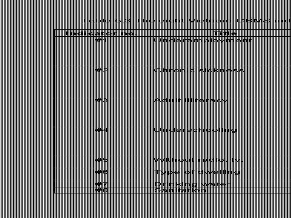
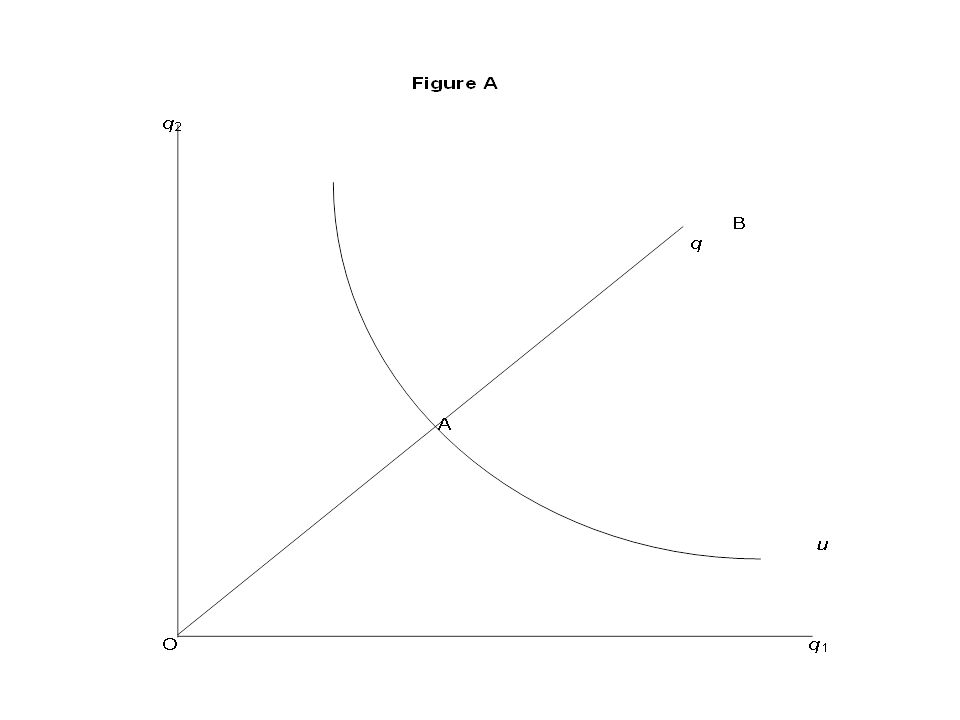


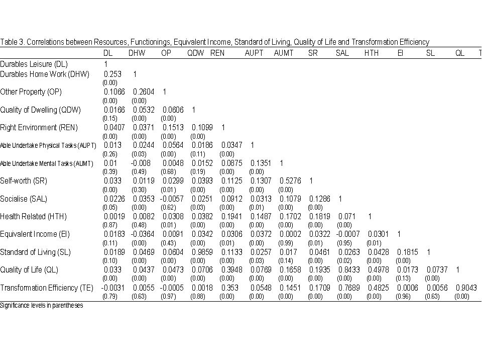

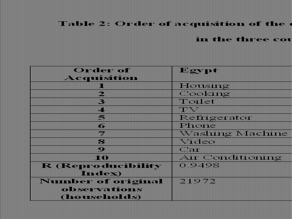


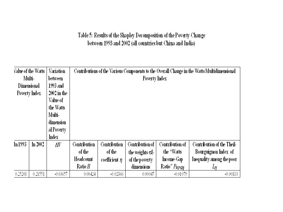


 Slideshow: prediction Original citation: Dougherty, C. (2012) EC220 - Introduction.>")


