Download presentation
Presentation is loading. Please wait.

1
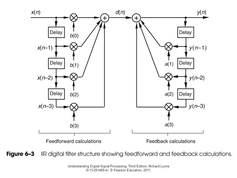
Infinite Impulse Response (IIR) Filters Uses both the input signal and previous filtered values y[n] = b 0 x[n] + b 1 x[n-1] + b 2 x[n-2] + … + a 1 y[n-1] + a 2 y[n-2] + a 3 y[n-3] + … The b k coefficients comprise the FIR part; filtering the input signal The a k coefficients comprise the IIR part; additional filtering using previously filtered values This concept has overlap with neural networks, a popular algorithm that statistically “learns” Sometimes called recursive filters
![Infinite Impulse Response (IIR) Filters Uses both the input signal and previous filtered values y[n] = b 0 x[n] + b 1 x[n-1] + b 2 x[n-2] + … + a 1 y[n-1] + a 2 y[n-2] + a 3 y[n-3] + … The b k coefficients comprise the FIR part; filtering the input signal The a k coefficients comprise the IIR part; additional filtering using previously filtered values This concept has overlap with neural networks, a popular algorithm that statistically learns Sometimes called recursive filters](http://images.slideplayer.com/13/4035569/slides/slide_1.jpg "Infinite Impulse Response (IIR) Filters Uses both the input signal and previous filtered values y[n] = b 0 x[n] + b 1 x[n-1] + b 2 x[n-2] + … + a 1 y[n-1] + a 2 y[n-2] + a 3 y[n-3] + … The b k coefficients comprise the FIR part; filtering the input signal The a k coefficients comprise the IIR part; additional filtering using previously filtered values This concept has overlap with neural networks, a popular algorithm that statistically learns Sometimes called recursive filters")
2
IIR Filter Code public static double[] convolution(double[] signal, double[] b, double[] a) { double[] y = new double[signal.length + b.length - 1]; for (int i = 0; i < signal.length; i ++) { for (int j = 0; j < b.length; j++) { if (i-j>=0) y[i] += b[j]*signal[i - j]; } if (a!=null) { for (int j = 1; j < a.length; j ++) { if (i-j>=0) y[i] -= a[j] * y[i - j]; } } return y; }
![IIR Filter Code public static double[] convolution(double[] signal, double[] b, double[] a) { double[] y = new double[signal.length + b.length - 1]; for (int i = 0; i < signal.length; i ++) { for (int j = 0; j < b.length; j++) { if (i-j>=0) y[i] += b[j]*signal[i - j]; } if (a!=null) { for (int j = 1; j < a.length; j ++) { if (i-j>=0) y[i] -= a[j] * y[i - j]; } } return y; }](http://images.slideplayer.com/13/4035569/slides/slide_2.jpg "IIR Filter Code public static double[] convolution(double[] signal, double[] b, double[] a) { double[] y = new double[signal.length + b.length - 1]; for (int i = 0; i < signal.length; i ++) { for (int j = 0; j < b.length; j++) { if (i-j>=0) y[i] += b[j]*signal[i - j]; } if (a!=null) { for (int j = 1; j < a.length; j ++) { if (i-j>=0) y[i] -= a[j] * y[i - j]; } } return y; }")
3
Characteristics of Recursive Filters Advantages –Powerful filtering with very few parameters –Execute very fast Example 1: b 0 =.15 and a 1 =.85 Example 1: b 0 = 0.93 b 1 = -0.93 a 1 = 0.86 Input Signal Example 1 output Example 2 output 0.0 1.0

4
Low and High Pass Recursive Filter Low Pass: b 0 = 1-x, a 1 = x High Pass: b 0 = (1+x)/2, b 1 = -(1+x)/x, a 1 = x 0≤x≤1, which controls the low and high pass boundaries
/2, b 1 = -(1+x)/x, a 1 = x 0≤x≤1, which controls the low and high pass boundaries")
5
Understanding Digital Signal Processing, Third Edition, Richard Lyons (0-13-261480-4) © Pearson Education, 2011.
 © Pearson Education, 2011.")
7
IIR Disadvantages float x = 1 for (int i=0; i<N; i++) { float a=Math.random(); float b=Math.random(); x = x + a; x = x + b; x = x - a; x = x - b; } Loops Error Do you see the flaws in the above program? Can be unstable: y n = x n + y n-1 //running sum Additive errors propagate (round off drift) Possible non-linear group delay
 Possible non-linear group delay.")
8
IIR Moving Average Filter Illustration (Sum of seven previous samples) y[50] = x[47]+x[48]+x[49]+x[50]+x[51]+x[52]+x[53] y[51] = x[48]+x[49]+x[50]+x[51]+x[52]+x[53]+x[54] = y[50] + x[54] – x[47] Example: {1,2,3,4,5,4,3,2,1,2,3,4,5}; M = 4 –Starting filtered values: {¼, ¾, 1 ½, 2 ½, … } –Next value: y 4 = 2 ½ + (5 – 1)/4 = 3 ½ Filter of degree (length) M –Centered Version: y n = y n-1 + x n+(M-1)/2 - x n-(M-1)/2 – 1 –Non Centered Version: y n = y n-1 + x n /M –x n-M /M Two additions per point no matter the filter length Note: Integers work best with this approach to avoid round off drift
![IIR Moving Average Filter Illustration (Sum of seven previous samples) y[50] = x[47]+x[48]+x[49]+x[50]+x[51]+x[52]+x[53] y[51] = x[48]+x[49]+x[50]+x[51]+x[52]+x[53]+x[54] = y[50] + x[54] – x[47] Example: {1,2,3,4,5,4,3,2,1,2,3,4,5}; M = 4 –Starting filtered values: {¼, ¾, 1 ½, 2 ½, … } –Next value: y 4 = 2 ½ + (5 – 1)/4 = 3 ½ Filter of degree (length) M –Centered Version: y n = y n-1 + x n+(M-1)/2 - x n-(M-1)/2 – 1 –Non Centered Version: y n = y n-1 + x n /M –x n-M /M Two additions per point no matter the filter length Note: Integers work best with this approach to avoid round off drift](http://images.slideplayer.com/13/4035569/slides/slide_8.jpg "IIR Moving Average Filter Illustration (Sum of seven previous samples) y[50] = x[47]+x[48]+x[49]+x[50]+x[51]+x[52]+x[53] y[51] = x[48]+x[49]+x[50]+x[51]+x[52]+x[53]+x[54] = y[50] + x[54] – x[47] Example: {1,2,3,4,5,4,3,2,1,2,3,4,5}; M = 4 –Starting filtered values: {¼, ¾, 1 ½, 2 ½, … } –Next value: y 4 = 2 ½ + (5 – 1)/4 = 3 ½ Filter of degree (length) M –Centered Version: y n = y n-1 + x n+(M-1)/2 - x n-(M-1)/2 – 1 –Non Centered Version: y n = y n-1 + x n /M –x n-M /M Two additions per point no matter the filter length Note: Integers work best with this approach to avoid round off drift")
9
Transforms Procedure –Transform the problem into a different domain –Execute a simpler algorithm in the transformed space –Transform back to get the solution DSP Example: We need a well-defined way to determine IIR filter coefficients that result in a filter that performs properly Image Processing : Mapping a three dimensional image into two dimension Some problems are difficult (or impossible) to solve directly
 to solve directly")
10
Laplace Transform The Fourier domain is a one dimensional space; each point represents a sinusoid of a particular frequency The Laplace domain (S- Domain) is a two dimensional space of complex numbers; each point represents sinusoids of a particular frequency that either amplifies with higher y-axis values or degrades with lower y-axis values Works with continuous functions. Positive frequency sinusoid Negative frequency sinusoid Fourier Domain Laplace Domain Positive frequency sinusoid that amplifies at a positive rate Positive frequency sinusoid that exponentially decay (attenuates) Imaginary axis Real axis
 Imaginary axis Real axis.")
11
The S-Domain 1.Each S-Domain point models a basis function 2.The top half is a mirror image of the bottom Real axis Imag axis Note: The waveforms are counterintuitive since filters convolute from the current time backward. Attenuating waves, actually produces unstable filters

12
Laplace Transform Example The Fourier transform is the Laplace Transform when σ=0

13
Laplace Transform Consider a process whose characteristics change over time Some function governs the changing behavior of the process We observe the process as a signal measured at points of time We want to predict the outputs, when the input system interacts with a filtering system process. We can model this problem with a differential equation, where time is the independent variable: a 1 y ’’’(t) + a 2 y’’(t) + a 3 y’(t) = b 1 x’(t) +b 2 x 2 x(t) A technique for solving differential equations
 + a 2 y’’(t) + a 3 y’(t) = b 1 x’(t) +b 2 x 2 x(t) A technique for solving differential equations.")
14
Laplace Transform Definition s is a complex number (σ+jω) where σ controls the degree of exponential decay and ω controls the frequency of the basis function e -st = e -(σ+jω)t = e -jωt / e σt The denominator controls the decay rate The numerator controls the frequency The integral starts if we are not interested in negative time (time past) dt
 where σ controls the degree of exponential decay and ω controls the frequency of the basis function e -st = e -(σ+jω)t = e -jωt / e σt The denominator controls the decay rate The numerator controls the frequency The integral starts if we are not interested in negative time (time past) dt")
15
Understanding Digital Signal Processing, Third Edition, Richard Lyons (0-13-261480-4) © Pearson Education, 2011. Impact of σ, ω values on the resulting basis function Assuming σ is negative

16
Poles and Zeroes The integrations causes S-plane some points to: –Evaluate to 0 (these are zeroes) –Evaluate to ∞ (these are poles) Pole and zero points determine IIR filter coefficients Note: Designing a filter comes down to picking the pole and zero points on the S-plane dt
 –Evaluate to ∞ (these are poles) Pole and zero points determine IIR filter coefficients Note: Designing a filter comes down to picking the pole and zero points on the S-plane dt")
17
An S-domain Plot Note The poles are the peaks The zeroes are the valleys Note: The third dimension is the magnitude of ∫ f(t)e -st dt at s = (σ+jω)
e -st dt at s = (σ+jω)")
18
Understanding Digital Signal Processing, Third Edition, Richard Lyons (0-13-261480-4) © Pearson Education, 2011.
 © Pearson Education, 2011.")
20
Time domain impulse response

21
Understanding Digital Signal Processing, Third Edition, Richard Lyons (0-13-261480-4) © Pearson Education, 2011. Attenuating impulse response Amplifying impulse response

22
The Low Pass Filter Illustration Transform the rectangular time domain pulse into the frequency domain and Into the s-domain

23
S-domain for a notch filter Fourier frequencies are the points where the real value is zero Notation x = pole ○ = zero

24
The z-transform Z-transform is the discrete cousin to the Laplace Transform Laplace Transform (s = σ+jω) – Extends the Fourier Transform, uses integrals and continuous functions – s = e -(σ+jω)t becomes the Fourier transform when ω = 0 – Fourier points fall along the imaginary axis – S-domain stable region is on the negative half of the domain Z-Transform (z = re -2 π k/t s ) – Extends the Discrete Fourier Transform, uses sums and discrete samples – z = e -j2πk/t s becomes the Discrete Fourier Transform (t s =sample size) – Four transform points fall along the unit circle – Z-domain stable domain are those within the unit circle Z{x[n]} =
![The z-transform Z-transform is the discrete cousin to the Laplace Transform Laplace Transform (s = σ+jω) – Extends the Fourier Transform, uses integrals and continuous functions – s = e -(σ+jω)t becomes the Fourier transform when ω = 0 – Fourier points fall along the imaginary axis – S-domain stable region is on the negative half of the domain Z-Transform (z = re -2 π k/t s ) – Extends the Discrete Fourier Transform, uses sums and discrete samples – z = e -j2πk/t s becomes the Discrete Fourier Transform (t s =sample size) – Four transform points fall along the unit circle – Z-domain stable domain are those within the unit circle Z{x[n]} =](http://images.slideplayer.com/13/4035569/slides/slide_24.jpg "The z-transform Z-transform is the discrete cousin to the Laplace Transform Laplace Transform (s = σ+jω) – Extends the Fourier Transform, uses integrals and continuous functions – s = e -(σ+jω)t becomes the Fourier transform when ω = 0 – Fourier points fall along the imaginary axis – S-domain stable region is on the negative half of the domain Z-Transform (z = re -2 π k/t s ) – Extends the Discrete Fourier Transform, uses sums and discrete samples – z = e -j2πk/t s becomes the Discrete Fourier Transform (t s =sample size) – Four transform points fall along the unit circle – Z-domain stable domain are those within the unit circle Z{x[n]} =")
25
Compare S-plane to Z-plane (cont.) Filter design S: analog filters; Z: IIR filters Equations S: differential equations, Z: difference equations Filter Points S: rectangular along i axis, Z: polar around unit circle Frequencies S: -∞ to ∞ (frequency line). Z: 0 to 2 π (frequency circle) Plots S and Z: Upper and lower half are mirror images Looking down vertically from the top of the domain Note: the Lines to left of s-plane correspond to circles within the unit circle in the z-plane Negative frequencies Positive frequencies
 Plots S and Z: Upper and lower half are mirror images Looking down vertically from the top of the domain Note: the Lines to left of s-plane correspond to circles within the unit circle in the z-plane Negative frequencies Positive frequencies.")
26
Understanding Digital Signal Processing, Third Edition, Richard Lyons (0-13-261480-4) © Pearson Education, 2011.
 © Pearson Education, 2011.")
28
Analog Filter Example σ=(A-3)/2RC; ω=±(A 2 +6A-5) ½ /2RC Sallen-Key Filters on a circle of 1/RC radius A = amplification R= resistance C = capacitance
/2RC; ω=±(A 2 +6A-5) ½ /2RC Sallen-Key Filters on a circle of 1/RC radius A = amplification R= resistance C = capacitance")
29
ButterWorth Filters ButterWorth poles are equally spaced around the left side of a circle

30
Example Low Pass Filters Butterworth poles are equally spaced on a circle Chebshev poles are equally spaced on an ellipse Elliptic poles are on an ellipse; zeroes added to the stopband north and south of the poles

31
Examples rφPolesa1a2 0.80.750.58±0.54j1.17-1.64 0.81.00.43±0.67j0.86-0.64 0.81.250.25±0.76j0.50-0.64 0.81.50.056±0.78j0.11-0.64 x x x x x x x x FreqBandwthrφPoles F13002500.950.120.963±0.116j F222002500.950.860.619±0.719j F330002500.951.170.370±0.874j x x x x x x There are tables of pole/zero points and their effects

32
Pole Placement Poles characterized by: – Amplitude: height of the resonance – Frequency: placement in the spectrum – Bandwidth: Sharpness of the pole Place pole at re iφ – Amplitude and bandwidth shrink as r approaches the origin 3-db down (half power) estimate = -2 ln(r) or 2(1-r)/r ½ – ω controls the resonant frequency When ω ≠0, IIR coefficients will be complex numbers IIR coefficients real if there are conjugate pairs (re iφ,re -iφ ) If r < 0.5, the relationship between φ and frequency breaks down because the pole “skirts” cause results to be less precise
 estimate = -2 ln(r) or 2(1-r)/r ½ – ω controls the resonant frequency When ω ≠0, IIR coefficients will be complex numbers IIR coefficients real if there are conjugate pairs (re iφ,re -iφ ) If r < 0.5, the relationship between φ and frequency breaks down because the pole skirts cause results to be less precise")
33
Transfer Function 1.IIR Definition: y n = b 0 x n + b 1 x n-1 +…+ b M x n-M + a 1 y n-1 +…+ a N y n-N 2.Z transform both sides: Y z =Z{b 0 x n +b 1 x n-1 +…+b M x n-M +a 1 y n-1 +…+a N y n-N } 3.Linearity Property: Y z = Z{b 0 x n }+Z{b 1 x n-1 }+…+Z{b M x n-M }+Z{a 1 y n-1 }+…+Z{a N y n-N } 4.Time delay property (Z{x n-k } = x z z -k ) Y z = b 0 X z + b 1 X z z -1 +…+b n-M X z z -M + a 1 Y z z -1 +…+a N Y z z -N 5.Gather Terms Y z - a 1 Y z z -1 -…- a N Y z z -N = b 0 X z + b 1 X z z -1 +…+ b n-M X z -M Y z (1- a 1 z -1 -…- a N z -N ) = X z (b 0 + b 1 z -1 +…+ b n-M z -M ) 6.Divide to get transfer function Y z /X z = H z = (b 0 + b 1 z -1 +…+ b n-M z -M )/(1- a 1 z -1 -…- a N z -N ) Y z = X z (Y z /X z ) = X z (H z ) // H z is the transform function for the filter 7.Perform Inverse Z transform: y[n] = x[n] * filter[n] // where * is convolution Because Z domain multiplication is time domain convolution A polynomial equation that defines filter coefficients for particular Z,S domain setting Starting with the IIR definition, derive Z-Transform Transfer Function Z{x[n]} =
![Transfer Function 1.IIR Definition: y n = b 0 x n + b 1 x n-1 +…+ b M x n-M + a 1 y n-1 +…+ a N y n-N 2.Z transform both sides: Y z =Z{b 0 x n +b 1 x n-1 +…+b M x n-M +a 1 y n-1 +…+a N y n-N } 3.Linearity Property: Y z = Z{b 0 x n }+Z{b 1 x n-1 }+…+Z{b M x n-M }+Z{a 1 y n-1 }+…+Z{a N y n-N } 4.Time delay property (Z{x n-k } = x z z -k ) Y z = b 0 X z + b 1 X z z -1 +…+b n-M X z z -M + a 1 Y z z -1 +…+a N Y z z -N 5.Gather Terms Y z - a 1 Y z z -1 -…- a N Y z z -N = b 0 X z + b 1 X z z -1 +…+ b n-M X z -M Y z (1- a 1 z -1 -…- a N z -N ) = X z (b 0 + b 1 z -1 +…+ b n-M z -M ) 6.Divide to get transfer function Y z /X z = H z = (b 0 + b 1 z -1 +…+ b n-M z -M )/(1- a 1 z -1 -…- a N z -N ) Y z = X z (Y z /X z ) = X z (H z ) // H z is the transform function for the filter 7.Perform Inverse Z transform: y[n] = x[n] * filter[n] // where * is convolution Because Z domain multiplication is time domain convolution A polynomial equation that defines filter coefficients for particular Z,S domain setting Starting with the IIR definition, derive Z-Transform Transfer Function Z{x[n]} =](http://images.slideplayer.com/13/4035569/slides/slide_33.jpg "Transfer Function 1.IIR Definition: y n = b 0 x n + b 1 x n-1 +…+ b M x n-M + a 1 y n-1 +…+ a N y n-N 2.Z transform both sides: Y z =Z{b 0 x n +b 1 x n-1 +…+b M x n-M +a 1 y n-1 +…+a N y n-N } 3.Linearity Property: Y z = Z{b 0 x n }+Z{b 1 x n-1 }+…+Z{b M x n-M }+Z{a 1 y n-1 }+…+Z{a N y n-N } 4.Time delay property (Z{x n-k } = x z z -k ) Y z = b 0 X z + b 1 X z z -1 +…+b n-M X z z -M + a 1 Y z z -1 +…+a N Y z z -N 5.Gather Terms Y z - a 1 Y z z -1 -…- a N Y z z -N = b 0 X z + b 1 X z z -1 +…+ b n-M X z -M Y z (1- a 1 z -1 -…- a N z -N ) = X z (b 0 + b 1 z -1 +…+ b n-M z -M ) 6.Divide to get transfer function Y z /X z = H z = (b 0 + b 1 z -1 +…+ b n-M z -M )/(1- a 1 z -1 -…- a N z -N ) Y z = X z (Y z /X z ) = X z (H z ) // H z is the transform function for the filter 7.Perform Inverse Z transform: y[n] = x[n] * filter[n] // where * is convolution Because Z domain multiplication is time domain convolution A polynomial equation that defines filter coefficients for particular Z,S domain setting Starting with the IIR definition, derive Z-Transform Transfer Function Z{x[n]} =")
34
Understanding Digital Signal Processing, Third Edition, Richard Lyons (0-13-261480-4) © Pearson Education, 2011.
 © Pearson Education, 2011.")
35
Transfer Function Example Suppose – b 0 =0.389, b 1 =-1.558, b 2 =2.338, b 3 =-1.558, b 4 =0.389 – a 1 =2.161, a 2 =-2.033, a 3 =0.878, a 4 =-0.161 Transfer Function H[z] = 0.389 - 1.558z -1 +2.338z -2 -1.558z -3 +0.389z -4 / (1-2.161z -1 + 2.033z -2 -0.878z -3 +0.161z -4 ) = 0.389z 4 - 1.558z 3 +2.338z 2 -1.558z 1 +0.389 / (z 4 -2.161z 3 + 2.033z 2 -0.878z 1 +0.161) Find the roots = (z-z 1 )(z-z 2 )(z-z 3 )(z-z 4 ) / (z-p 1 )(z-p 2 )(z-p 3 )(z-p 4 ) Note: The bottom form tells us where the zeroes and poles are
![Transfer Function Example Suppose – b 0 =0.389, b 1 =-1.558, b 2 =2.338, b 3 =-1.558, b 4 =0.389 – a 1 =2.161, a 2 =-2.033, a 3 =0.878, a 4 = Transfer Function H[z] = z z z z -4 / ( z z z z -4 ) = 0.389z z z z / (z z z z ) Find the roots = (z-z 1 )(z-z 2 )(z-z 3 )(z-z 4 ) / (z-p 1 )(z-p 2 )(z-p 3 )(z-p 4 ) Note: The bottom form tells us where the zeroes and poles are](http://images.slideplayer.com/13/4035569/slides/slide_35.jpg "Transfer Function Example Suppose – b 0 =0.389, b 1 =-1.558, b 2 =2.338, b 3 =-1.558, b 4 =0.389 – a 1 =2.161, a 2 =-2.033, a 3 =0.878, a 4 = Transfer Function H[z] = z z z z -4 / ( z z z z -4 ) = 0.389z z z z / (z z z z ) Find the roots = (z-z 1 )(z-z 2 )(z-z 3 )(z-z 4 ) / (z-p 1 )(z-p 2 )(z-p 3 )(z-p 4 ) Note: The bottom form tells us where the zeroes and poles are")
36
Understanding Digital Signal Processing, Third Edition, Richard Lyons (0-13-261480-4) © Pearson Education, 2011.
 © Pearson Education, 2011.")
37
Notch Filter Z 1 = 1.00 e i(π/4), Z 2 = 1.00 e i(-π/4) P 1 =0.9e i(π/4), P 2 =0.9e i(-π/4) Z 1 =0.7071+0.7071i Z 2 =0.7071-0.7071i P 1 =0.6364+0.6364i P 2 =0.6364-0.6364i 1.Convert to rectangular form 2.Multiply the complex polynomials 3.Collect terms 4.Use the coefficients for the filter Note: Compare to the s-plane example
, Z 2 = 1.00 e i(-π/4) P 1 =0.9e i(π/4), P 2 =0.9e i(-π/4) Z 1 = i Z 2 = i P 1 = i P 2 = i 1.Convert to rectangular form 2.Multiply the complex polynomials 3.Collect terms 4.Use the coefficients for the filter Note: Compare to the s-plane example")
38
Understanding Digital Signal Processing, Third Edition, Richard Lyons (0-13-261480-4) © Pearson Education, 2011. Second-order low pass IIR filter examples

39
Understanding Digital Signal Processing, Third Edition, Richard Lyons (0-13-261480-4) © Pearson Education, 2011.
 © Pearson Education, 2011.")
41
Linear filters can be combined into parallel or serial systems

42
Understanding Digital Signal Processing, Third Edition, Richard Lyons (0-13-261480-4) © Pearson Education, 2011. Note: It’s easier to design multiple two tap systems than a larger multiple tap system

43
Understanding Digital Signal Processing, Third Edition, Richard Lyons (0-13-261480-4) © Pearson Education, 2011. Original Gain: (b 0 +b 1 )/(1 - a 1 ) = 0.22 + 0.25 / (1-0.87) = 3.614 Do normalize gain, divide coefficients by 3.64
/(1 - a 1 ) = / (1-0.87) = Do normalize gain, divide coefficients by")
Similar presentations


 Sogang University Department of Mechanical Engineering.>")


 can be.>")


 Filters>")


: Impulse sampler, Laplace.>")
![Z-Transform Fourier Transform z-transform. Z-transform operator: The z-transform operator is seen to transform the sequence x[n] into the function X{z},](/17/5301252/big_thumb.jpg "Z-Transform Fourier Transform z-transform. Z-transform operator: The z-transform operator is seen to transform the sequence x[n] into the function X{z},>")

 Kevin D. Donohue Electrical and Computer Engineering University of Kentucky.>")