1. Interspecific Competition
There are many forms of interaction between/among populations. Before focusing on interspecific competition let’s quickly review the full spectrum of interactions. One of the best ways is to consider the impact of interactions on the component populations:
donor population
mutualism commensalism predation…
recipient pop neutralism
amensalism competition
Of these interactions, intensive research has basically concentrated on competition and predation/herbivory.

2. Competition was believed to be the key factor regulating populations from the early 1960s until ~1980. Why?
The ‘stars’ (MacArthur, Connell, May,…) thought so. As in most fields, it is difficult to reject the dominant view and still be successful in getting grants and publications.
2. One seminal paper had singular influence over ecological thinking. That paper is still fondly called “The Etude”. It was so important, you should think critically about what it said. It is a paper written in broad-stroke generalities. In the end we will reject those generalities (the devil is in the details), but first allow yourself to be swept up by them.

3. The Etude: Hairston, Smith and Slobodkin (1960) Community
structure, population control, and competition. Am. Nat.
94:421-5.
Hairston, et al. first observe that in contemporary
communities fossil fuels are accumulating at a negligible rate compared to the amount of photosynthesis occurring world-wide. If decomposing plant material is not accumulated, then it is being used up. Decomposers, as a trophic level, are limited by their food resources.
If that's true, then species in the decomposer trophic level must, on average, be competing for those limited food resources.

4. 2. Consider the producer (plant) trophic level. From our
earthly point of view plants seem (quoting the paper)
'abundant and largely intact'. Only in exceptional, non-
natural conditions is over grazing or large scale destruction
of the plant community evident. There are natural
occasions, but they are spatially and temporally rare.
Similarly, weather catastrophes do not usually destroy large
areas of plant community. On average, then, the world is
green.
3. If so, then plants are not limited from above by their
herbivores, nor by catastrophic weather, yet we are not
overrun by plants. They must then be limited by resources
(space, light, nutrients) and compete for those resources.

5. 4. If 'the world is green', then herbivores are clearly not limited
by their food resources; those are present in abundance.
Some herbivores may, at some times, be controlled by
weather or the abundance of plant food, but Hairston, et al.
argue that those are exceptional cases. They suggest that
significant herbivore damage to vegetation occurs most
frequently when non-native herbivores are introduced.
Those introduced species are the ones least likely to be
adapted to local weather conditions, and therefore most
likely to be controlled by them. Since non-natives are the
species which most damage plant communities, weather is,
on average, an unacceptable explanation for control. If
neither resources nor weather control herbivores, but they
do not usually increase to plague levels, then they are
controlled, and predators must be the cause.

6. 5. Finally, consider predators (and parasites by association). If
predators successfully control herbivore numbers, then they
limit their own food supply, and must, as food-limited
species, compete for the limiting resource. Territoriality,
most common among predator species, is an adaptation to
protect sufficient resource to ensure survival.
The conclusions of The Etude are, therefore, that of four trophic levels, 3 are controlled (regulated?) by competition: decomposers, producers, and predators; only one is not regulated by competition, the herbivores.
Since then, we’ve learned that the world was not so green as Hairston, et al. claimed; plants have an enormous variety of structural and chemical defenses which, more or less frequently, limit herbivore populations.

7. We’ve also learned how important predation can be in structuring communities. Predators active at the time of flowering and seed maturation can dramatically alter plant success. Keystone predators alter species composition and relative abundance of prey communities.
To begin to think about competition as a limiting and/or regulating factor, recognize that all populations that are resource limited must undergo intraspecific competition. We’ll begin there.
competition acts as a controlling agent only when its ultimate effect is to decrease the contribution of competing individuals to future generations below that which would have been made had there been no competition, i.e. it must have impact on fitness.

8. 2. competition only occurs when some resource necessary to survival and/or reproduction is present only in a limited supply.
3. in most cases competition is a bi-directional interaction, i.e.
each competing individual has impact on the success of all
with whom it competes, and is mutually affected by its
competitors. The interaction need not, however, be
symmetrical; there can be dominant and subordinate
individuals in an interaction, with unequal effects on each
other. 
4. Competition is density dependent, i.e. the probability of an individual being affected, and/or the intensity of effects of interaction, increase with the density (or number) of individuals in the population.

9. When intraspecific competition occurs, it is seen as taking two forms, and two types of characterizations have been developed:
Nicholson, in his studies of sheep blowflies, defined the two extreme forms. He called those extremes 'scramble' and 'contest‘ competition.
More recently an alternative division separates categories called 'interference' and 'exploitation‘ competition.
There are similarities between the two categorizations.

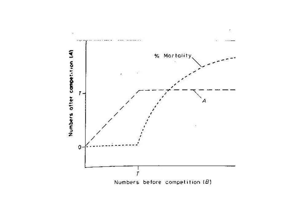
10. Contest/Scramble
Scramble competition assumes a different distribution of resources than does contest interaction. At low densities all individuals get sufficient resource to grow at a maximum rate (i.e. lx and mx are unaffected by interaction).
While rates (growth, survivorship, and fecundity) decline with increasing density, in scramble competition all individuals continue to get an equal share of resources as density
increases. Therefore, above some threshold density each individual gets less resource than it needs to maintain an R0 of 1; individuals do not survive and/or reproduce successfully, and the population decreases to 0.
Graphically:

12. In scramble competition it is assumed that the interaction is symmetrical. On the other hand, in contest competition the interactions are asymmetrical. Some individuals win in competitive contests with others. For simplicity, we assume that the winners each have equal abilities, and similarly the losers. Losers get no resources above the threshold, but
winners get an equal share of the resource base. Above the threshold only winners survive, and their number is fixed by the resource base; all others die.
In scramble competition all individuals produce an optimal mx below threshold density, but above it, with insufficient resources, all have a 0 mx.
In contest competition, winners continue to reproduce at optimal levels, while losers cease reproduction.

14. Interference/Exploitation
In interference, one part of a population (or one species) prevents access of the other to a resource, while consuming only its own needs.
Resources are sequestered by those who are successful at interference. Like contest competition, the winners function as if unaffected by competition, while the losers die.
Exploitation’s effects are not absolute at any threshold. In this case both kinds (populations, species) use resources with (usually) different efficiencies. The presence of the competitor lowers the resource use of each species, and therefore its success, but, unless competitive exclusion occurs or there are no alternative resources, both persist with increased mortality and/or decreased fecundity in the short term.

15. The relative abilities or resource use efficiencies of the species involved determine how symmetrical or asymmetrical the interaction is.
If competition is asymmetrical (or in the traditional Lotka-Volterra description, 12  21 with equal Ks) then the equilibrium condition is the presence of only the stronger competitor).
For example, 2 species of bumblebees are each, when alone, able to exploit 2 flower species (a larkspur and a monkshood). The length of their probosces and the length of the corollas on the two flowers are different. When both bees are present, each depletes the nectar resources of the flowers on which it is the more efficient forager to levels which make the resource effectively useless for the other.

16. Exploitation interactions produce a competitive exclusion (Inouye 1978) based on competitive asymmetry with respect to each of the two resources.
But does competition “regulate” populations?
What does “regulation” mean?

17. The classic example that shows competition can regulate population is Nicholson’s laboratory studies of sheep blowflies…
The adult sheep blowfly, Lucilia cuprina, lays its eggs on sheep carcasses or meat, and the meat is the food source for larval development. In addition, the amount of meat available for a larva determines its egg laying potential. The adult also feeds on carcass meat. While the results are the same, Nicholson, in separate experiments:
gave adults surplus food (no competition) but limited food available to larvae, or
offered larvae unlimited food resources (no competition), but gave adults a limited food resource.
The same sort of cycles resulted in each case.

18. Let's follow the results when adults were given surplus food: 
  when adults have surplus food  
large numbers of adults high egg production  
pupation increases many larvae
more food available food depleted per larva (limited food available)
proportion successfully
fewer eggs are produced pupating is low
adult population declines reduced recruitment into
the adult population

19. This scheme is obviously cyclic
This scheme is obviously cyclic. It produces population cycles with a period of days, and the cycling is caused by 'regulation' due to competition among larvae.
A key problems with Nicholson's sorting out of competition (and the separation into contest and scramble forms of competition) is the insistence upon threshold density levels associated with qualitative changes in growth, reproduction, or survivorship as density passes through that threshold. Real experiments show little evidence of such a threshold, at least one leading to qualitative change. Instead, most competition experiments seem to find gradual increase in interactive
effects as density increases.

20. Much of the best quantitative data measuring effects of competition comes from studies of plants. A paper by Palmbald (1968), for example, expressly deals with population size results, rather than the more usual measures of 'yield‘ in studies of agricultural plant competition.
Palmbald studied a variety of weeds, most annual, so that seed output was a measure of population growth. What he found was differing kinds of response in different species, but a
tendency for the weedy annuals to have plasticity in reproduction, and perennials to have plasticity in growth parameters.

21. Capsella bursa-pastoris (shepherd’s purse) is fairly typical of annuals. Germination and pre-reproductive mortality show only slight responses, but the size of individuals and the number of seeds produced per individual are strongly affected by density.
Seed production falls dramatically, from 23,000 at 1 plant per pot to 210 at 200 per pot, that is by a factor of about 100. Close to parallel is the decline in biomass per plant. Thus, the allocation of biomass to produce seeds is relatively constant, measured as the number of seeds per gram individual plant biomass.
The data follows:

22. Sowing density
% germination
% mortality
% reproducing
% vegetative
Dry weight (g)
Dry weight/plant
Seeds/repro
ducing individual
Total seeds

23. There are two things going on:
One is measured at the individual level, where growth, size, and reproduction change approximately in proportion to density over fairly wide ranges.
The other is reproductive output per unit area. This is the measure important to agriculture. A farmer wants to maximize his yield per acre, while minimizing his costs (here seeds planted). Since seminal papers in the 1950's it has been clear that there is a maximum production per unit area. Below some 'threshold' density the total production increases
toward that maximum; above it plasticity (an almost universal characteristic of plant growth and reproduction) reduces the growth, etc. of individuals and maintains that maximum. Plants 'compensate' for density changes, and the result is the 'law of constant final yield' (Kira,et al. 1953,Yoda et al. 1958).

24. Bromus grown in
pots
Corn grown in a
field

25. Do plants exactly compensate for density?
The answer is no. Plants 'undercompensate' at low densities, and totals increase. At higher densities they frequently 'overcompensate', i.e. totals do not remain exactly constant, but decrease slightly. That’s what was evident in the data for Capsella.
The growth of Bromus follows what would be called compensation, but seed production at very low plant densities cannot reach the maximum yield.
The growth of corn shows ‘overcompensation’, in that total grain yield declines at very high densities.

26. Also note the impact of different fertilizer levels
Also note the impact of different fertilizer levels. The maximum yield increases in Bromus when additional nitrogen fertilizer is added. In general, the maximum yield is set by environmental conditions, both biotic (e.g. weed occurrence and density) and abiotic (climate, soil nutrients).
Compensation develops over time.
When plants start growth, the biomass density is low, and total
biomass in pots increases with further growth (which could be
described as 'undercompensation' if yield were measured at each time by the total biomass of plants).
However, as they grow, biomass density increases, until is approaches the maximum. If we look at yield-density curves over time, they begin as straight lines, yield increasing in proportion to density.

27. At mid-season the relationship maintains the same slope at low density, but curves over to flatten at the maximum when plants are at a higher density. Late in the season the curve has reached its aymptote at all densities, and is flat.