2. Multi Dimensional Steady State Heat Conduction P M V Subbarao Associate Professor Mechanical Engineering Department IIT Delhi It is just not a modeling but also feeling the truth as it is…

3. Heat treatment of Metal bars & rods

4. Heat Flow in Complex Geometries (Casting Process)

5. Microarchitecture of Pentium 4

6. Thermal Optimization of Microarchitecture of an IC Microprocessor power densities escalating rapidly as technology scales below 100nm level. There is an urgent need for developing innovative cooling solutions. The concept of power-density aware thermal floor planning is a recent method to reduce maximum on-chip temperature. A careful arrangement of components at the architecture level, the average reduction in peak temperature of 15°C. A tool namely, Architectural-Level Power Simulator (ALPS), allowed the Pentium 4 processor team to profile power consumption at any hierarchical level from an individual FUB to the full chip. The ALPS allowed power profiling of everything, from a simple micro- benchmark written in assembler code, to application-level execution traces gathered on real systems. At the most abstract level, the ALPS methodology consists of combining an energy cost associated with performing a given function with an estimate of the number of times that the specific function is executed.

7. The energy cost is dependent on the design of the product, while the frequency of occurrence for each event is dependent on both the product design and the workload of interest. Once these two pieces of data are available, generating a power estimate is simple: multiply the energy cost for an operation (function) by the number of occurrences of that function, sum over all functions that a design performs, and then divide by the total amount of time required to execute the workload of interest.

8. Need for Thermal Optimization

9. Thermal Management Mechanism in Pentium 4 The Pentium 4 processor implements mechanisms to measure temperature accurately using the thermal sensor. In the case of a microprocessor, the power consumed is a function of the application being executed. In a large design, different functional blocks will consume vastly different amounts of power, with the power consumption of each block also dependent on the workload. The heat generated on a specific part of the die is dissipated to the surrounding silicon, as well as the package. The inefficiency of heat transfer in silicon and between the die and the package results in temperature gradients across the surface of the die. Therefore, while one area of the die may have a temperature well below the design point, another area of the die may exceed the maximum temperature at which the design will function reliably. Figure is an example of a simulated temperature plot of the Pentium 4 processor.

11. Thermal Optimization of Floor Plan Initial ModelLow Cooling cost Model

12. General Conduction Equation For Rectangular Geometry: Conduction is governed by relatively straightforward partial differential equations that lend themselves to treatment by analytical methods if the geometries are simple enough and the material properties can be taken to be constant. The general form of these equations in multidimensions is:

13. 0 W H x y Steady conduction in a rectangular plate Boundary conditions: x = 0 & 0 < y < H : T(0,y)= f 0 (y) x = W & 0 < y < H : T(W,y)= f H (y) y = 0 & 0 < x < W : T(x,o)= g 0 (x) y = H & 0 < x < W : T(x,H)= g W (x)

14. Write the solution as a product of a function of x and a function of y: Substitute this relation into the governing relation given by

15. Rearranging above equation gives Both sides of the equation should be equal to a constant say l 2

16. Above equation yields two equations The form of solution of above depends on the sign and value of l 2. The only way that the correct form can be found is by an application of the boundary conditions. Three possibilities will be considered:

17. Integrating above equations twice, we get The product of above equations should provide a solution to the Laplace equation: Linear variation of temperature in both x and y directions.

18. i.e. l 2 = -k 2 Integration of above ODEs gives: &

19. Solution to the Laplace equation is: Asymptotic variation in x direction and harmonic variation in y direction

20. i.e. l 2 = k 2 Integration of above ODEs gives: &

21. Solution to the Laplace equation is: Harmonic variation in x direction and asymptotic variation in y direction.

22. Summary of Possible Solutions

23. Steady conduction in a rectangular plate 2D SPACE – All Dirichlet Boundary Conditions 0 W H x y T = T 1 T = T 2 Define: Laplace Equation is: q = 0 q = C

24. l 2 =0 Solution

25. Simultaneous Equations The solution corresponds to l 2 =0, is not a valid solution for this set of Boundary Conditions!

26. l 2 0 Solution OR 0 W H x y q = 0 q = C l 2 > 0 is a possible solution ! Any constant can be expressed as A series of sin and cosine functions.

27. Substituting boundary conditions :

29. Where n is an integer. Solution domain is a superset of geometric domain !!! Recognizing that

30. where the constants have been combined and represented by C n Using the final boundary condition:

31. Construction of a Fourier series expansion of the boundary values is facilitated by rewriting previous equation as: where Multiply f(x) by sin(mp x/W) and integrate to obtain

32. Substituting these Fourier integrals in to solution gives:

33. And hence Substituting f(x) = T 2 - T 1 into above equation gives:

34. Therefore

35. Isotherms and heat flow lines are Orthogonal to each other!

36. Linearly Varying Temperature B.C. 0 W H x y q = 0 q = Cx

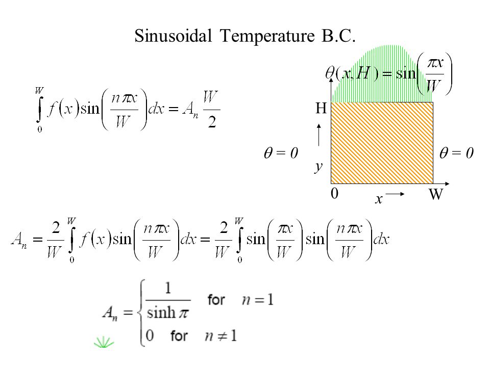
38. Sinusoidal Temperature B.C. 0 W H x y q = 0 q = Cx

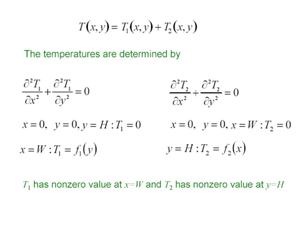
40. Principle of Superposition P M V Subbarao Associate Professor Mechanical Engineering Department IIT Delhi It is just not a modeling but also feeling the truth as it is…

43. For the statement of above case, consider a new boundary condition as shown in the figure. Determine steady-state temperature distribution.

46. Where n is number of block. If we assume  y =  x, then:

47. If m is a total number of the heat flow lanes, then the total heat flow is:

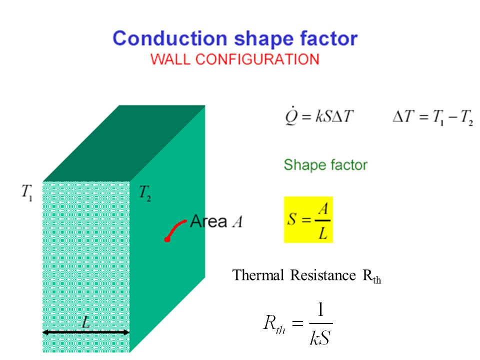
49. Thermal Resistance R th

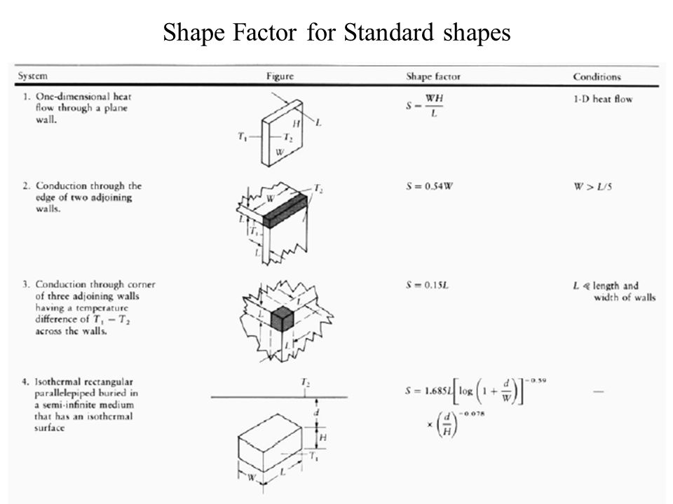
53. Shape Factor for Standard shapes

56. Thermal Model for Microarchitecture Studies Chips today are typically packaged with the die placed against a spreader plate, often made of aluminum, copper, or some other highly conductive material. The spread place is in turn placed against a heat sink of aluminum or copper that is cooled by a fan. This is the configuration modeled by HotSpot. A typical example is shown in Figure. Low-power/low-cost chips often omit the heat spreader and sometimes even the heat sink;

57. Thermal Circuit of A Chip The equivalent thermal circuit is designed to have a direct and intuitive correspondence to the physical structure of a chip and its thermal package. The RC model therefore consists of three vertical, conductive layers for the die, heat spreader, and heat sink, and a fourth vertical, convective layer for the sink-to- air interface.

58. Multi-dimensional Conduction in Die The die layer is divided into blocks that correspond to the microarchitectural blocks of interest and their floorplan.

59. For the die, the Resistance model consists of a vertical model and a lateral model. The vertical model captures heat flow from one layer to the next, moving from the die through the package and eventually into the air. R v2 in Figure accounts for heat flow from Block 2 into the heat spreader. The lateral model captures heat diffusion between adjacent blocks within a layer, and from the edge of one layer into the periphery of the next area. R 1 accounts for heat spread from the edge of Block 1 into the spreader, while R 2 accounts for heat spread from the edge of Block 1 into the rest of the chip. The power dissipated in each unit of the die is modeled as a current source at the node in the center of that block.

60. Thermal Description of A chip The Heat generated at the junction spreads throughout the chip. And is also conducted across the thickness of the chip. The spread of heat from the junction to the body is Three dimensional in nature. It can be approximated as One dimensional by defining a Shape factor S. If Characteristic dimension of heat dissipation is d