Download presentation
Presentation is loading. Please wait.

1
Compiling sunspot catalogue: the princeples Lajos Győri Heliophysical Observatory of the Hungarian Academy of Sciences, Gyula Observing Station

2
In the Debrecen Heliophysical Observatory we comply a sunspot catalogue (Debrecen Photoheliographic Data, DPD) as a continuation of Greenwich Photoheliographic Results (GPR). The basic data in a sunspot catalogue are the heliographic positions and the areas of the sunspots. So our task is to automate the determination of them. The determination of the borders of the sunspots amounts to the determination of their position and area: the area is the number of the pixels inside the border and the position is the center of gravity of pixels inside the border weighted by the their intensities. As a sunspot can be divided into two distinct area (umbra and penumbra) we must determine two borders, one for the penumbra and another for the umbra.
 we must determine two borders, one for the penumbra and another for the umbra..")
3
Probably the first idea that comes into mind when solving the task of looking boundaries in an image is the use of the gradient image. High values of the gradient indicate the presence of a border, an abrupt change in the gray-level value. In the figure we can see that the garadient image contains a lot of information about the boundaries but it cannot be directly interpreted as photosphere-penumbra and penumbra-umbra border. The trouble with the gradient image in our case is that the gradients along the boundaries do not represent a contiguous, clearly cut closed line mainly due to the filamentary structure being present in a sunspot group as it can be sen in the figure.

4
The photospheric noise can be decreased by global thresholding (if the gradient value of a pixel is lower than a threshold value, then the gradient of this pixel is set to zero). Applying a local thresholding (retaining the gradient value of a pixel only if it is local maximum inside a prescribed enviroment of the pixel in question) the surplus gradients can be decreased even more. But, as it can be seen in the figure, it does not solve the problem. Here we applied a global thresholding using the gadient value two standard deviation above the mean gradient and a local thresholding with a 9x9 enviroment. One imaginable workaround is to look for additional filtering mechanism and, at the same time, an algorithmwhich patches the inceasing gaps in the prospective border of the spots.
 the surplus gradients can be decreased even more. But, as it can be seen in the figure, it does not solve the problem. Here we applied a global thresholding using the gadient value two standard deviation above the mean gradient and a local thresholding with a 9x9 enviroment. One imaginable workaround is to look for additional filtering mechanism and, at the same time, an algorithmwhich patches the inceasing gaps in the prospective border of the spots..")
5
I have chosen another approach to make use of the information contained in the gradient image. Let us assign a gradient value to every intensity contour (the term contour here means isodensity line) of the image by summing up the gradient along points of the contour and dividing the sum by the number of the contour pixels. Let AGAC (average gradient along contour) denote this value. It is reasonable (at least as a first approximation) to choose the contour having maximum AGAC among the contours of the spot as the penumbra- umbra border of the spot. Similarly the contour having first local maximum in AGAC among the contours of the spot can be taken as the photosphere-penumbra boundary of the spot. : Gradient at the ith pixel of the contour N: Number of the pixels along the contour
 of the image by summing up the gradient along points of the contour and dividing the sum by the number of the contour pixels. Let AGAC (average gradient along contour) denote this value. It is reasonable (at least as a first approximation) to choose the contour having maximum AGAC among the contours of the spot as the penumbra- umbra border of the spot. Similarly the contour having first local maximum in AGAC among the contours of the spot can be taken as the photosphere-penumbra boundary of the spot. : Gradient at the ith pixel of the contour N: Number of the pixels along the contour.")
6
The left figure below shows the variation of AGAC along the contours of the spot S shown in the right figure. Contours are indexed by their intensity. S phot. - pen. baundary pen. - umb. baundary

7
It can occur that different part of the border of sunspot have different intensities. The seeing can also distort the intensity along the boundary of a sunspot. To make allowances for these, a refinement of the above definition of the spot boundary is needed. It can be done as fallows. The preliminary boundary obtained in the first approximation is divided into sectors. The average gradient along a sector of the preliminary boundary is compared to the values of the average gradient along adjacent sectors of several neighboring contours and the sector of the preliminary boundary is replaced by the one having the maximum average gradient value.

8
It is a general technique of the image processing to decompose the image somehow (analyzing stage) and after that to use this decomposition to gain the features to be found in the image (synthesizing stage). If we want to make use of the idea stated above then the decomposition of the solar image into contour set presents itself. This contour set contains the borders of the spots and, moreover, reflects the structural relationships between spots. The accompanying figure illustrates this contour set superimposed on the image.

9
Correcting for limb darkening Now let's see how these ideas can be casted in a program which determines the areas and the heliographic positions of the sunspots from the solar image and the data characterizing the circumstances of it's taking. The main stages of the program are as follows: Findig the solar limb points: in order to determine the center of the solar disk and the disk radius. These parameters are needed to transform the disk coordinates of the spots into heligraphic coordinates. Determining the alignment of the image: the angle between the columns of the image and the sun's axis of rotation Removing artifacts: - cross-threads, - double exposed parts

10
Removing large scale variations from the image: - clouds, - developing unevenness, - spatial variation of the trans-illuminating light. Determining the statistics of the photosphere: - mean, - standard deviation. They are used to determine the initial intensity and the incremental step intensity for the contour set. The purpose is to save computer time. Determining the gradient image Decomposing the imge into a contour set

11
Picking out the contours for every preliminary spot from the contour set. A preliminary spot is local maximum (we use the inverse image) that have at least one contour in the contour set. Here we olso pick out the contours of the holes (photospheric material inside a penumbra). Determining the photosphere-penumbra and penumbra-umbra boundaries of the spots. Spots having the same penumbra-umbra boundary are merged into an umbra in regard their area but their positions are retained. Arranging the preliminary spots into penumbras and umbras Filtering out: - granular spots, - emulsion defect, - artifacts, - darker regions in the penumbra, - umbral unevenness
 that have at least one contour in the contour set. Here we olso pick out the contours of the holes (photospheric material inside a penumbra). Determining the photosphere-penumbra and penumbra-umbra boundaries of the spots. Spots having the same penumbra-umbra boundary are merged into an umbra in regard their area but their positions are retained. Arranging the preliminary spots into penumbras and umbras Filtering out: - granular spots, - emulsion defect, - artifacts, - darker regions in the penumbra, - umbral unevenness.")
12
Improving the photosphere-penumbra and penumbra-umbra boundaries. Up to this time, the boundaries of the spots were iso-intensity lines. Here we apply the method described above to improve the accuracy of the borders. Determining the position and areas of the spots from their boundaries. When determining the penumbral areas the effect of the holes are taken into account.

15
Let's take the gradient image of the solar image and put a circle on it. Let's determine the mean gradient picked up by the perimeter of the circle. Repeating this process with systematically changed circle parameters (radius and center position) we can find the circle parame- ters that maximize the mean gradient along the circle. The circle points are in the vicinity of the limb but its accuracy is not too high. We can help it as follows. Let's draw a straight line segment across every circle pixels perpendicularly to the circle. Taking the profile along the line segments in the image (the original, not the gradient), we can find the inflexion points on the limb. Several artifact (fluffs, scratches, defects) can occur near the limb showing up as outsiders among the limb pixels. They are filtered out.
 we can find the circle parame- ters that maximize the mean gradient along the circle. The circle points are in the vicinity of the limb but its accuracy is not too high. We can help it as follows. Let s draw a straight line segment across every circle pixels perpendicularly to the circle. Taking the profile along the line segments in the image (the original, not the gradient), we can find the inflexion points on the limb. Several artifact (fluffs, scratches, defects) can occur near the limb showing up as outsiders among the limb pixels. They are filtered out..")
16
But the seeing induced undulation of the limb is retained. After that a median smoothing is applied. The accompanying figures are the snapshots of this process. In the bottom most figure the cross-thread is already filtered out. The width of the yellow limb line coresspods to about 0.5 arcsec on the sky. A note is in order. Originally the solar disk is a circle. Due to the refraction the limb become undulated and ellipse. Approaching to the horizon, the eccentricity of the ellipse is increasing. So, in extreme case, it is better (but slower) to substitute the circle in the above process for an ellipse.
 to substitute the circle in the above process for an ellipse..")
17
Also, this is the case when we are not sure that the enlargements along the rows and the columns of the image, provided by the scanner is accurate enough. It is deserve to mention that the method is not suscetibile to intensity variations along the limb as it can be seen in the figure, which is a part of a cloudy photoheliogram. The same method that is used to determine the boundary of the spots can be applied to find the limb, too. But it is sensitive to larger intensity variations along the limb. I use this method when I have a part image not knowing if it contains the solar limb because it is faster.

18
The algorithm: - A copy of the original image is created (I original1 ). - Image I original1 is smoothed i.e. a pixel is replaced with the average of the pixels within a given environment (I smoothed ). - Image I smoothed is subtracted from the original image (I subtracted ). - We look for uneven regions in image I subtracted. We come to this later - A second copy of the original image is created (I original2 ). - The parts of I original2 that correspond to the uneven regions of I subtracted are replaced by the average of the neighboring even regions of I subtracted (I patched ). - Image I pacthed is smoothed (I ps ). - Image I ps is subtract from the original image. The image obtained this way will be the image corrected for large scal variation. In essence, we subtract the large scale background from the image, but before doing so we find the regions of the image that does not belong the background.
. - Image I smoothed is subtracted from the original image (I subtracted ). - We look for uneven regions in image I subtracted. We come to this later - A second copy of the original image is created (I original2 ). - The parts of I original2 that correspond to the uneven regions of I subtracted are replaced by the average of the neighboring even regions of I subtracted (I patched ). - Image I pacthed is smoothed (I ps ). - Image I ps is subtract from the original image. The image obtained this way will be the image corrected for large scal variation. In essence, we subtract the large scale background from the image, but before doing so we find the regions of the image that does not belong the background..")
19
The algorithm to find uneven regions in the image: - A grid is superimposed on image I subtract. - The mean intensity and the standard deviation inside every cell of the grid is determined. - A sub-grid of 3x3 is superimposed on every cell of the grid. - The mean intensity and the standard deviation inside every cell of the sub-grid is determined. - Let's form the following quantities on the grid cells DI=AI max -AI min, DS=SI max -SI min, where AI max : maximum average intensity on the sub-grid, AI min : minimum average intensity on the sub-grid, SI max : maximum STD on the sub-grid, SI min : minimum STD on the sub-grid, - if( (DI/SI min > L 1 ) || (DS/SI min > L 2 ) || (SI/SI min ]) > L 3 ) then the cell is uneven, where L 1, L 2 and L 3 are appropriate constants, in our case: L 1 =2.5, L 2 =1.2, L 3 =1.8.
 || (DS/SI min > L 2 ) || (SI/SI min ]) > L 3 ) then the cell is uneven, where L 1, L 2 and L 3 are appropriate constants, in our case: L 1 =2.5, L 2 =1.2, L 3 =1.8..")
Similar presentations
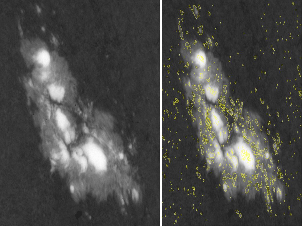

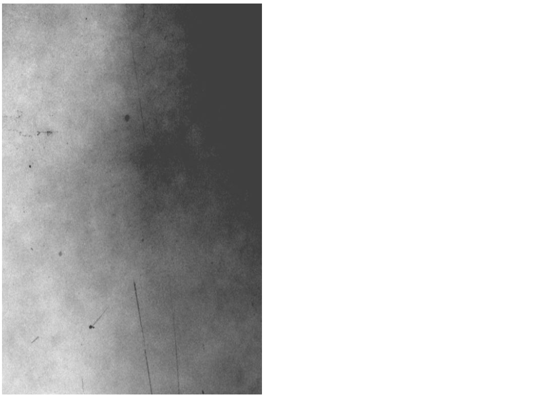


Image pre-processing.>")


