1. Previous version of notes: PK Basu
ECO 120- Macroeconomics
Weekend School #2
9th June 2007
Lecturer: Rod Duncan
Previous version of notes: PK Basu

2. Topics for discussion Module 4- The role of the government
The tools the Australian government controls to smooth short-run fluctuations in the economy
Module 5- Macroeconomic applications
The link between inflation and unemployment, economic growth and Australian trade with the rest of the world
What will not be discussed
Answers to Assignment #2 (use the CSU forum for this)

3. Money Money has three main functions in the economy.
Money is a medium of exchange. We use exchange money when we buy/sell to each other.
Money is a unit of account. Money is an agreed measure for stating the value of other goods and services.
Money is a store of value. Money can be kept under the bed or inside a jar and used to exchange for goods and services in the future.

4. Official measures of money
M1 is the amount of notes and coins (“currency”) in circulation plus current deposits with banks.
M3 is M1 plus all other bank deposits.
Credit cards are not counted as money, since using a credit card is accumulating debt, whereas deposits at a bank can be turned into money without accumulating debt.

5. Money multiplier
What happens when you take $1 cash to a bank to deposit it?
(1) You deposit the cash in the bank, and the bank creates an account for you with $1 in it.
Money = $1
(2) The bank doesn’t keep the cash. Instead the bank has to keep R, called the “reserve ratio” (0 < R < 1), of the $1 as reserves and then loans out $(1 - R).
(3) The person who receives the loan of $(1-R) spends the cash, and the merchant who receives the $(1-R) puts that in his bank. This increases the merchant’s account by $(1-R).
Money = $1 + $(1-R)

6. Money multiplier
(4) The second bank keeps $R(1-R) as reserves and loans out $(1-R)(1-R) = $(1-R)2 as new loans.
Money = $1 + $(1-R) + $(1-R) 2 + …
If this process continues, the value of money created is 1/R = 1 + (1-R) + (1-R)
So for every $1 floating in the economy in currency, we have $1/R in currency plus deposits in the economy. This ratio m = 1/R is called the “simple money multiplier”. For every $1 in currency that the government prints, the money supply increases by m.

7. Equilibrium in the money market
Equilibrium in the money market means supply of money equals demand for money.
Supply of money
The supply of money depends on the level of currency in the economy and the money multiplier. The supply of money does not depend on the interest rate.
Demand for money
People require money to make purchases, ie. How much currency is in your pocket?

8. Demand for money
The higher is income and prices, the greater the amount of money required to make the purchases people will wish to make.
But a $1 in your pocket is a $1 not in the bank. In the bank, that $1 would be accumulating interest, but in your pocket, it accumulates no interest. So the interest rate is the price of holding money as currency rather than as a deposit in the bank. So we would expect that as the interest rate rises, people will lower the level of currency that they hold.
The demand for money is downward-sloping in the interest rate, i, and increases in income and prices.

9. Equilibrium in the money market
The supply of money does not depend on the interest rate, so it is vertical.
The interest rate is the price of holding wealth as currency, so money demand falls as i rises.

10. Monetary policy
The government can control the supply of money and thus the interest rate. These actions are called “monetary policy”.
“Open market operations” are a means of the government controlling the supply of money. The government (in our case the Reserve Bank of Australia or RBA) buys and sells government securities, such as government bonds to control the amount of money in the economy.
If the RBA buys a bond with currency, the RBA increases the money supply (by the change in currency times the money multiplier).

11. Monetary policy
If the RBA sells bonds for currency, it decreases the supply of money.
Monetary policy shifts the money supply curve and so changes the equilibrium interest rate.

12. Monetary policy
“Monetary policy” is the government operation of the money supply and interest rates.
Typically we consider the problem of how the government can manipulate monetary policy so as to control economic variables such as output, inflation, interest rates, etc.
Issues: how monetary policy can “stabilize” the economy? how will monetary policy affect interest rates or exchange rates?

13. Who operates monetary policy?
The Reserve Bank of Australia (RBA) is responsible for monetary policy.
The RBA was given 3 goals when it was created:
Maintain low inflation
Maintain low unemployment
Maintain value of the A$
The RBA was only given one policy tool- the money supply to achieve 3 goals. In the mid 1990s, the RBA was simply told to have one aim:
Maintain low inflation- “inflation target” of 2-3%.

14. Definitions
The RBA implements monetary policy through its control of the cash rate.
Cash rate: The cash rate is the rate the RBA charges bank for loans within the RBA reserves system. The cash rate is the base interest rate for the economy, and all other interest rates are derived from it.
Easy monetary policy: When the RBA lowers the cash rate to stimulate AD.
Tight monetary policy: When the RBA raises the cash rate to cut off AD.

15. Interest rates
As we saw in the Investment section, the profitability of investment projects depends on the nominal interest rate.
The lower are interest rates, the more projects will be profitable, so the higher will be investment spending.
Since the RBA controls the cash rate, and since all interest rates depend on the cash rate, the RBA controls I, and so can shift the AD curve.

16. How monetary policy works
Cause–Effect Chain of Monetary Policy:
RBA cash rate impacts interest rates
Interest rates affect investment
Investment is a component of AD
Equilibrium GDP is changed

17. Easy Monetary Policy SF1 SF2 10 8 6 10 8 6 Investment demand D110 8 6
Investment
demand D1
Amount of investment, i
AD1 AS
Easy Monetary Policy
Price level
AD2 Y

18. Tight Monetary Policy SF2 SF1 10 8 6 10 8 6 Investment demand D110 8 6
Investment
demand D1
Amount of investment, i AS
Tight Monetary Policy
Price level
AD1
AD2
Real domestic output, GDP

19. Inflation targeting
The RBA makes known their target or desired level of inflation- 2-3% inflation.
The RBA will tighten monetary policy, raise i, if inflation appears to be too high.
The RBA will loosen monetary policy, lower i, if inflation appears to be too low.
The RBA has to “look ahead” to the level of future inflation.

20. Inflation targeting How can we put this into our AD-AS model? P Y2007
100
AD2007
AS2007
103
102
Target band
AD2008
AS2008
RBA raises i

21. Monetary policy and the open economy
Net Export Effect
Changes in interest rate affect the value of the exchange rate under floating exchange rate. An increase in interest rate appreciates the currency, resulting in lower net exports
A decrease in interest rate leads to currency depreciation and a rise in net exports
So an easy monetary policy is enhanced by the net export effect.

22. Sample exam question QUESTION : B.3
Using the models from our subject, carefully explain the consequences if the government reduces the supply of paper money (or “cash”) by an amount, m.
a) What are the consequences on the total level of money?
b) What are the consequences in the money market?
c) What are the consequences in the AD-AS model for the economy as a whole?

23. Quantity theory of money
There is a nice, simple model of money which explains many features of money supply and demand. This model is called the quantity theory of money.
If we imagine that money is needed for all of the purchases made each year, then demand for money is the vale of purchases: PY.
The supply of money for purchases is the amount of cash in the economy.
But each piece of money in the economy can be used multiple times during a year in transactions. We call the number of transactions the velocity of money “v”.

24. Quantity theory of money
So the total supply of money for transactions in a year is v times M: vM.
So demand equals supply requires that:
PY = vM
So if Y goes up, but nothing else does, then average level of prices must fall.
The QTM is good to use for thinking about money and inflation.

25. Fiscal policy
“Fiscal policy” is the government operation of government spending (G) and taxes (T).
Typically we consider the problem of how the government can manipulate G and T so as to control economic variables such as output, inflation, interest rates, etc.
Issues: how fiscal policy can “stabilize” the economy? what about government borrowing and public debt?

26. Definitions
Budget deficit: the budget deficit is the extent of overspending by the government
Budget deficit = G – T
Expansionary fiscal policy: increasing the budget deficit (G↑ or T↓) usually in a recession.
Contractionary fiscal policy: decreasing the budget deficit (G↓ or T ↑) usually in an economic boom.

27. Budget deficits and surpluses
If the government spends more than it brings in in taxes, what happens? (G > T)
The money has to come from somewhere. For developed countries, this means borrowing (issuing government debt or “public debt”) from domestic residents or foreigners.
If the government is spending less than it brings in in taxes, the government can reduce public debt. The Australian government has followed this policy in the last 10 years.

28. Types of fiscal policy We differentiate two types of fiscal policy:
Discretionary fiscal policy: This is fiscal policy that comes about from planned changes in G and T that the government brings in in response to the economic situation.
Non-discretionary fiscal policy: This is fiscal policy that comes about from the design of spending and taxes. There is no government official actively determining these changes.

29. Non-discretionary fiscal policy
Certain parts of our spending and taxes automatically increase demand in a recession (when AD < potential GDP) and decrease demand in a boom (when AD > potential GDP).
Welfare spending and unemployment benefits are part of G and increase in a recession and decrease in a boom.
Income and company taxes are part of T and depend on GDP, they increase during a boom and decrease during a recession.
These act as “automatic stabilizers” on the economy, reducing the variability of the economy.

30. Cyclically-adjusted budget deficits
The automatic stabilizers raise the budget deficit in a recession and lower the budget deficit in a boom.
This fact means that we can not just look at the budget deficit to determine whether the government is “overspending”, we also have to take into account where we are in the business cycle.
Adjusting the budget deficit for the point we are in the business cycle is called “cyclically adjusting”. We would expect even a “sensible” government to be in a deficit in a recession.

31. Stabilizing a boom Y Y0 AD AS P Yn
LR AS

32. Stabilizing a recessionY Y0 AD AS P Yn
LR AS

33. Discretionary fiscal policy
Discretionary fiscal policy is the manipulation of G and T by government officials typically to reduce the severity of shocks to the economy.
It sounds like a good idea, but how does it work in reality?
There are many problems and limitations to the use of fiscal policy to reduce recessions and booms.

34. Problems with discretion
Scenario: Imagine a train driver that has only one control- an accelerator/brake that he or she can push or pull on to control the train. This is exactly the same situation as the government faces with fiscal policy.
Now what limitations can the train driver face?

35. Train driver problem
GDP
Time
June
August

36. Problems with discretion
Limitations:
Correctness of data: Is the train driver seeing the tracks correctly? Or Does the government get the right data about where the economy is?
Timing of data: Is the train driver seeing the tracks with enough time to react? Or Does the government get the statistics quickly enough to do anything?
Decision lags: Can the train driver make a decision about the correct action before the train reaches the problem spot? Or does the government have time to design the correct fiscal policy?

37. Problems with discretion
Administration lags: If the driver pulls on the control, how long will it take for the brakes to start to work? Or New spending and taxes have to be passed through parliament, which takes time, even after a decision is made.
Operational lags: If the brakes start to work, how long before the train slows down? Or New government spending and taxes take time to affect the economy.
So even the best-designed fiscal policies can go wrong if they are in response to the wrong data or if they take too long to affect the economy.

38. Political considerations
There are further concerns we might have about the operation of fiscal policy.
Politicians have to remain popular. No one likes taxes, and everyone likes new spending on themselves. Will a politician make an unpopular decision that may result in them losing the election if it is the best decision for the economy.
Electoral cycles: Governments have to be re-elected every 3-4 years. So a politician would love to engineer a boom right before his or her election.

39. Crowding out
Another problem with fiscal policy is that an increase in G may increase output but at the expense of other components of aggregate expenditure.
Y = C + I + G + NX
Since the economy returns to potential GDP over the long-run, an increase in G must come at the expense of either C, I or NX or all 3.
If an increase in G reduces investment spending over the long-run, this could lead to lower future growth in the economy.

40. Crowding out How can this happen?
An increase in G shifts the AD curve to the right.
This results in higher Y and higher P.
The increased government borrowing in the market for savings raises the interest rate.
Higher interest rates lead to lower investment spending so I drops, shifting AD left.
Higher interest rates leads to an appreciation of the A$ (as foreign investors put their money in Australia), so NX drops, shifting AD left.

41. Crowding out- I and NX AS
ASLS
AD1 P3 P2 P1
AD3
AD2 Q1 Q2 Qp

42. Government debt
One problem that economic commentators always point to is the level of government debt- “Our debt is too high.”
How do we evaluate the level of government debt? How do we know is it is “too high”.
Government debt is like any other form of debt. You evaluate the debt relative to the income/wealth of the person incurring the debt.
A $500,000 debt might be high to you and me, but it might mean nothing to Kerry Packer.

43. Government debt
So we need to evaluate government debt relative to “government income”. But what is the appropriate form of “government income”, as the government doesn’t earn or produce anything.
Generally we use the income of the country as the comparison, since the government is free to tax or claim any part of GDP.

44. Government debt
So our criterion for “too much” is debt (B, since typically government debt is issued in government bonds) over GDP (Y):
B / Y
Banks would make much the same calculation when considering whether to issue someone a home loan.
In general debt is growing at the rate of interest each year, r, while GDP is growing at the growth rate of the economy, g.

45. Debt Comparison

46. Sample exam question 1 QUESTION : C.2
A balanced budget fiscal policy would require the government to spend more when the economy is in a boom (and taxes are high) and require the government to spend less when the economy is in a recession (and taxes are low).
(a) Explain the business cycle using the AD-AS model, assuming that it is changes to the AD curve that makes the cycle happen. Assume here that government spending is held constant over the business cycle.
(b) Explain the effect of a balanced budget fiscal policy on the business cycle using the AD-AS model.
(c) Is the balanced budget fiscal policy helping or hindering the economy?

47. Sample exam question 2 QUESTION : C.3
The monetarists believe that the aggregate supply (AS) curve is very steep, while the Keynesians believe the AS curve is flat.
(a) Explain how fiscal policy would work in each case in the aggregate demand-aggregate supply (AD-AS) model.
(b) What would you expect that the two camps have to say about the effectiveness of fiscal or monetary policy?

48. Unemployment A person becomes unemployed:
Job loser
Job leaver
New entrant or re-entrant into the labour force
He or she is no longer unemployed:
Hired or recalled
Withdraws from the labour force

49. Labour Force Participation Rate
Population
Working age population
Labour Force Participation Rate
Labour Force
Employed or
Unemployed
Unemployment Rate

50. Labour force participation rate
Proportion of country’s population that takes part in its economic activities directly (either actually taking part or willing to) /
Labour Force
Working Age Population X
100
LFPR In Australia, in September 2003 :
( million / million ) x 100 = %

51. Unemployment rate
Proportion of country’s labour force that is unemployed. ( / )
Number Unemployed
Labour Force X
100
UR in Australia, in September 2003 :
(0.591 million / million) x = 5.8%

52. Types of unemployment Three main types of unemployment:
Cyclical unemployment
Frictional unemployment
Structural unemployment

53. Cyclical unemployment
Associated with the ups and downs of the business cycle
Takes place due to insufficient aggregate demand or total spending- reflects shifts in AD curve.
High during recessions and low during booms.
Fiscal and monetary policies can reduce cyclical unemployment - policies are relevant.

54. Frictional unemployment
Associated with the period of time in which people are searching for jobs, being interviewed and waiting to commence duties.
It is inevitable and always exist
Fiscal and monetary policies can not reduce frictional unemployment – macroeconomic policies are irrelevant.
Policies that make it easier to find new jobs will affect frictional unemployment.

55. Structural unemployment
Associated with wider structural or technological changes in the economy that may make some jobs redundant.
It is inevitable and always exist
Lasts longer than frictional unemployment
Fiscal and monetary policies can not reduce structural unemployment – macroeconomic policies are irrelevant.
Policies that encourage workers to retrain skills or to move to a new area with more jobs will decrease structural unemployment.

56. “Full” employment
Full employment means when all productive resources in the economy are in full use - implies no cyclical unemployment - still frictional and structural unemployment exist - they can be low - but can never be zero.
The full-employment rate of unemployment is called the “natural rate of unemployment”.
Domestic output consistent with the natural rate of unemployment is “potential output” or “full employment level of GDP”.

57. Classical employment theory
Economy always operates under full employment - it is automatic and self sustaining - if there is any unemployment that is only temporary.
Price-wage flexibility
the assumption that all prices, including wages and interest rates, are flexible and will, rapidly adjust to remove disequilibria
Classical theory and laissez faire
the price system ensured that price-wage flexibility and fluctuations in the interest rate was capable of maintaining full employment

58. Classical theory P1
Price Level P2
AD1
AD2 Q1
Real Domestic Output

59. Keynesian employment theory
Full employment is not automatic - unemployment exists for longer periods - the Great Depression of the 1930s - sticky wages and prices.
Horizontal aggregate supply curve during recession - ‘recessionary’ or ‘Keynesian’ range.
Change in AD impacts on unemployment - not on price level.
Once the full employment level is reached - vertical AS curve - change in AD affects price level only.
Unstable aggregate demand - especially investment, so that demand management and stabilisation policies by the government are essential.

60. Keynesian theory AS P1
Price Level
AD1
AD2 Q2 Q1
Real Domestic Output

61. Sample exam question QUESTION : B.2
The government wants to spend money reducing unemployment. What effect on official unemployment statistics would the following policies have:
a) Increasing the unemployment benefit,
b) Lengthening the period during which people can get the unemployment benefit,
c) Funding more job-training programs, and
d) Increasing the funding for university enrolments.

62. Current year index - Previous year
Measuring inflation
We measure the general price level through a price index such as the Consumer Price Index (CPI)
Inflation is a continuous rise in the general price level. We measure inflation:
Inflation
rate
Current year index - Previous year
index
Previous year index x
100 =

63. Inflation in Australia, 1970-2004

64. Two types of inflation
We can differentiate two different sources of inflation in an economy:
Demand-Pull Inflation
Occurs when an increase in AD pulls up the price level.
Cost-Push Inflation
Occurs when an increase in the cost of production at each price level shifts the AS curve leftward resulting in increased prices.

65. Demand-pull inflation
Short-run: There is an increase in demand, such as an increase in consumer spending, so AD shifts rightward. AS does not change in the short run, and we have a movement along the AS curve. Price level and GDP increases..
Long run: Workers will realise their real wages have fallen and will demand and receive increased nominal wages. As costs rise, supply decreases and the AS to shift to the left. Price level increases, and GDP declines.
May be caused by expansionary fiscal and monetary policies - can be countered by contractionary policies by the government.

66. Demand-pull inflation- SR and LR
ASLR
Price Level
AS1
A decrease in
aggregate
supply....
Increases the price
level and output
returns to original
level P3 c P2 b P1 a
AD2
AD1
Real GDP o Q1 Q2

67. Cost-push inflation
Short-run: Increased prices and decreased real output (and more unemployment). Causes can be:
Wage push : increase in wage rate - power of trade unions
Supply shocks - increase in prices of major raw materials - oil etc.
Profit push : increase in profit requirement of large monopoly businesses.
The AS curve shifts to the left/up as prices and costs rise, and firms cut back on output.

68. Cost-push inflation Long-run: There are two scenarios.
Government intervention ( shift in AD): If government intervenes to increase AD, prices and output will rise, moving us back to the natural rate of output.
No Government intervention (no shift in AD): If government does not intervene to increase AD, a severe recession will result. However nominal wages will eventually decline and will restore AS to its original position, moving us back to the natural rate of output.

69. Cost-push inflation- SR and LR
ASLR
AS2
AS1
An attempt to
increase AD
will only further
increase the
price level P3 c b
Price Level P2 P1 a
AD1
Real GDP o Q1 Q2

70. Phillips curve
Suggests an inverse relationship (or a trade-off) between inflation and the unemployment rate
Named after A W Phillips who originally discovered the relationship between unemployment and nominal wages, using British data in 1950s.
In general, inflation is associated with economic expansion, and unemployment with economic recession.
During expansion : the greater the rate of growth of AD - inflation is high, and unemployment is low.
During recession : the slower the rate of growth of AD - inflation is low, and unemployment is high.

71. Phillips curve Annual rate of inflation (percent)7 6 5 4 3 2 1
Annual rate of inflation
(percent)
Unemployment rate (percent)

72. Policy implications of Phillips curve
Trade-off suggests : a rise in inflation should lead to a decline in unemployment, and vice versa.
In general, both can not be brought down to the minimum level.
The society must make a choice between low inflation and low unemployment.

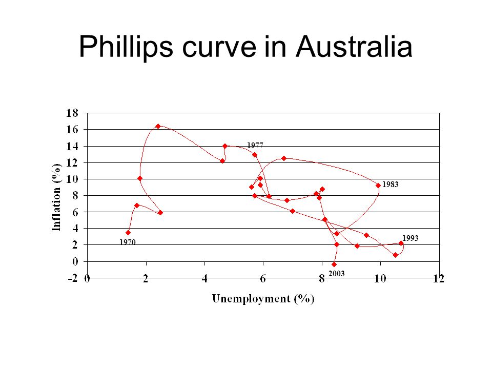
73. Phillips curve in Australia
1977
1983
1993
1970
2003

74. Stagflation
Simultaneous experience of high and increasing unemployment and inflation - cost-push inflation.
Caused by :
Aggregate supply shocks such as severe increases in fuel costs, and devaluations;
Productivity declines; or
Inflationary expectations and wages - expectations about the likely future path and rate of increase of the general price level.

75. Sample exam question QUESTION : C.4
(a) Carefully explain what the Phillips curve shows.
(b) Why did the experiences of the Australian economy in the 1970s seem to contradict the Phillips curve?
(c) How could the rise in oil prices in the early 1970s explain what we were observing with the Phillips curve?

76. Long-run growth
We are ultimately interested in the level of resources each individual in society has access to. The level of resources will then somewhat determine what opportunities each person has.
So we are ultimately interested in GDP per person of an economy. Growth is the increase of GDP per capita over time.
Y / N = output per person

77. Long-run growth
But not every person in an economy is “economically productive”, so if we want to link “worker productivity” and GDP per capita , we need:
Y / N = (Y/Nw) (Nw/N)
Y/Nw = output per worker depends on labour productivity, which depends on skills in workforce, capital, tech
Nw/N = labour force participation rate which depends on cultural attitudes and aging of the population

78. Labour force participation
Growth in GDP per capita can come from increasing Nw/N.
As people move from subsistence farming on rural areas to paid employment in urban areas, labour force participation rises.
As women move out of unpaid domestic work to paid domestic work, labour force participation rises.
But obviously there is a limit to this sort of growth.

79. Labour force participation

80. Labour force participation
And as the Australian population ages, we will eventually see this LFP start to decline, as the population of retirees increases.
This will be a major challenge for Australia in the relatively near future.

81. Output per worker
Output per worker, Y/Nw, is the main source of growth in Australia.
So growth in Australia depends on increasing the productivity of our workers. What determines how productive a worker is?
The skills of the worker.
The physical capital the worker uses.
The level of technology the worker and capital have access to.

82. Output per worker

83. Output per worker
Output per worker was $22,000 in 1950 and $52,000 in 2000 in constant dollars. (Once we remove the effects of inflation.)
So how are Australian workers today over twice as productive as workers in 1950?
New technologies (mechanization, robotics, computers, etc)
More capital (powered floor polishers instead of mops)

84. Output per capita
So once we combine labour force changes and worker productivity changes, we wind up with change in output per capita over time.
Real GDP per capita was $9,200 in 1950 and $25,500 in 2000.
Australians in 2000 have almost twice as much resources per person than Australians did in 1950.

85. Long-run growth in Australia

86. Long-run growth in Australia
While there was a temporary blip in GDP in early 1950s, 1980s and 1990s, the overall picture is one of steadily increasing GDP per person over time.
What can be done to ensure growth in Australia?
Increasing productivity per worker.
Increasing skill levels, increasing capital and increasing technology.

87. But remember…
Remember what it is that GDP measures: the market value of all goods and services sold in the economy.
Ignores non-market goods, such as domestic work and pollution.
Does not include black market goods.
Having longer holidays might make for a happier workforce, but would lower GDP.

88. Growth and economic development

89. What about other countries?
Relative to the rest of the developed world, Australia is a fast-growing economy.
Australia is behind the United States, but ahead of countries such as the UK and NZ.
Relative to our neighbours (East Asia), Australia is a very prosperous country.

90. Relative to developed countries

91. Relative to our neighbours

92. Convergence
“Convergence” is the idea that we would expect countries that are initially poorer should grow faster than countries that are richer.
Why?
Technology- Poor countries can piggy-back for free off the technology developed by rich countries.
Capital flow- We expect investors to rush to invest in countries with cheap wages.

93. Convergence
Over time, we expect poor countries to grow faster than rich countries, so GDP per capita across different countries should “converge” over time.
Is this idea true?
We saw that certain countries like Japan and South Korea started off poorer than Australia but caught up.

94. Catching up?

95. But look!

96. Consequences of growth
Life
Adult
Enrollment
GDP
Expectancy
Literacy
in Edu
per capita
HDI
Rank
Norway
78.5
100 97
29,918
0.942 1
Australia
78.9
116
25,693
0.939 5
USA 77 95
34,142 6
Japan 81 82
26,755
0.933 9
Indonesia
66.2
86.9 65
3,043
0.684
110
Kenya
50.8
82.4 51
1,022
0.513
134
Uganda 44
67.1 45
1,208
0.444
150
Malawi 40
60.1 73
615
0.4
163

97. Closed and open economies
A closed economy is one that does not interact with other economies in the world.
There are no exports, no imports, and no capital flows.
An open economy is one that interacts freely with other economies around the world.

98. An open economy
An open economy interacts with other countries in two ways.
It buys and sells goods and services in world product markets.
It buys and sells capital assets in world financial markets.
The Australian economy is a medium-sized open economy—it imports and exports relatively large quantities of goods and services.

99. Exports and imports
Exports are domestically produced goods and services that are sold abroad.
Imports are foreign produced goods and services that are sold domestically.
Net exports (NX) or the trade balance is the value of a nation’s exports minus the value of its imports.
NX = X - M

100. Net exports
A trade surplus is a situation where net exports (NX) are positive.
Exports > Imports
A trade deficit is a situation where net exports (NX) are negative.
Imports > Exports

101. Net Exports ( )
% of GDP
In A$

102. Net exports and domestic GDP
Aggregate Expenditure = C + I + G + X - M
Level of X depends on foreign countries’ income, not domestic income
Level of M is dependent on domestic income or GDP.

103. What affects net exports?
The tastes of consumers for domestic and foreign goods.
The prices of goods at home and abroad.
The exchange rates at which people can use domestic currency to buy foreign currencies.
The costs of transporting goods from country to country.
The policies of the government toward international trade.

104. Exchange rate
The exchange rate is the rate at which a person can trade the currency of one country for the currency of another.
The nominal exchange rate is expressed in two ways.
In units of foreign currency per one Australian dollar
In units of Australian dollars per one unit of the foreign currency

105. Exchange rate
At an exchange rate between the US dollar and the Australian dollar is 0.70 US cents to one Australian dollar.
One Australian dollar trades for 0.70 of US$. [This is the form we will use.]
One US$ trades for 1.43 (1/0.7) of an Australian dollar.

106. Determination of exchange rates
The market price of something is determined in the market.
Under the Floating Rate system, price of a currency (its exchange rate) in the international market for currency is determined by its demand and supply.
A$ is a floating currency - floated in December 1983.

107. Value of A$ ( )
Yen/A$
US$/A$

108. Determination of exchange rates
Demand for A$ (people who want to buy A$):
By overseas buyers of Australian goods and services (including their tourist visits to Australia)
By overseas investors who want to buy Australian physical and financial assets.
Supply of A$ (people who want to sell A$):
By Australian importers (including overseas trips by Australians)
By Australian investors who want to buy physical and financial assets overseas.

109. Appreciation/Depreciation
If a dollar buys more foreign currency, there is an appreciation of the dollar -- say, one A$ buys one US$ instead of 70 US cents at present.
If it buys less there is a depreciation of the dollar -- say, one A$ buys 50 US cents instead of 70 US cents at present.

110. Demand for A$
As exchange rate (US$ per A$) increases (say, from US$ 0.70 to US$ 1), exports become more expensive. Overseas buyers will buy less of Australian goods and services. Demand for A$ falls.
(Just opposite when the value of A$ decreases)
So, Demand curve for A$ (or any other currency) is downward sloping - as exchange rate increases, demand for the currency falls, and vice versa.

111. Supply of A$
As exchange rate increases (say, from US$ 0.70 to US$ 1), imports become cheaper. Australians will buy more of foreign (imported) goods and services. Supply of A$ increases.
(Just opposite when the value of A$ decreases)
So, Supply curve of A$ (or any other currency) is upward sloping - as exchange rate increases, supply of the currency increases,
and vice versa.

112. Determination of exchange rates
Exchange rate (cost of 1 A$ in terms of US$)
Supply of A$
Demand for A$
Amount of A$

113. Sample exam question QUESTION : C.1
World oil prices rise and are likely to stay high for the future. Assuming all else held constant:
(a) Explain the effects of a rise in the price of oil on Australia using the aggregate demand-aggregate supply (AD-AS) framework.
(b) Explain the effect of higher world oil prices on the Australian external accounts and the exchange rate.
(c) How would your answers to (a) and (b) change if the world’s second-largest oilfield was discovered southwest of Perth? Explain carefully.

114. Balance of payments
Reflected in international balance of payments accounts.
Records all transactions between the entities in Australia and those in foreign nations
Two basic accounts:
Current Account
Capital Account

115. Balance of payments
Current account of a country’s international transaction refers to the record of receipts from the sale of goods and services to foreigners (exports), the payments for goods and services bought from foreigners (imports), and also property income (such as interest and profits) and current transfers (such as gifts) received from and paid to foreigner.
Capital account is a summary of country’s asset transactions with the rest of the world.

116. Balance of payments = Capital Account Balance (+,-)
Current Account Balance (+,-)
= Capital Account Balance (+,-)
Demand for A$ equals Supply of A$.
If we have a current account deficit (we are importing more than we are exporting), then we must also have a capital account deficit (investors overseas are accumulating Australian assets).

117. Exact impact depends on relative strengths of the two opposing forces.
CAD (Current Account Deficit) and exchange rate
CAD impacts on :
Inflow of foreign investment - higher the CAD, higher the surplus in capital account - higher investment in Australia by the foreigners - higher the demand for A$.
Outflow of foreign currency - income (interest & profit) on foreign investment goes out of the country- higher the CAD, higher the demand for foreign currency - higher the supply of A$.
Exact impact depends on relative strengths of the two opposing forces.

118. Current Account Deficits (1949-1996)
% of GDP
In A$

119. Is the Current Account Deficit a Problem?
Represents a debt we will have to repay in the future.
Just as for a household, the extent of the problem depends on our ability to service the debt- but notice that CAD as a percentage of GDP (ability to service debt) is still low.

120. Sample exam question QUESTION : B.5
a) What is Australian foreign debt? How do we calculate it?
b) Why does it matter to economists that most of Australian foreign debt is held by firms and households (the private sector) rather than the government (the public sector)?

121. Terms of Trade
The ratio of average price of goods and services exported by a country to the average price of its imports.
If prices of imported goods are rising at a faster rate than the prices of exported goods, then the terms of trade for that economy is considered as deteriorating. The economy is loosing in the process of foreign trade.

122. Terms of Trade ( )

123. Purchasing Power Parity (PPP)
The purchasing-power parity theory is the simplest and most widely accepted theory explaining the variation of currency exchange rates.
According to the purchasing-power parity theory, a unit of any given currency should be able to buy the same quantity of goods in all countries.

124. Intuition for PPP
In an open economy, I have the choice of buying an orange in Australia or an orange from Indonesia and importing the orange back to Australia.
If transport costs are low, the price of traded goods should be the SAME, once we translate into a common currency.
This is called the law of one price.

125. Purchasing-Power Parity
Law of one price
When converted to a common currency value through the exchange rate, the price of identical goods should be the same across countries:
Pd = E x Po/s,
Where Pd is the domestic price, Po/s is the foreign price and E is the exchange rate.

126. Tips for preparing for the exam
Practice. Do the problems in the back of the book chapters. Do the problems on the book’s website. Do the problems in the study guide.
Read the question. Read carefully.
Answer the question. Don’t answer the question you think was asked. Answer the question that actually was asked. Most exam errors happen here. Remember to read the question.

127. Tips for preparing for the exam
Be sure to answer all of the question.
Don’t put down too much. Don’t provide a whole background of a model unless the question asks for it. If the question asks you to analyse a scenario, go straight into the scenario.
Don’t put down too little. In an essay question, provide your reasoning and analysis. Draw a relevant graph and talk about the graph. Don’t just say “Yes.”

128. Final exam tip
Don’t panic! Relax and breath. You do not need to write for 3 hours to do well in an economics exam. Often a well-ordered sentence is worth more than 2 pages of semi-coherent babbling. Stop and think about your answer.