Cellular Wireless Networks

Cellular Wireless Networks
Chapter 10

Introduction (1) Cellular technology
is the foundation of mobile wireless communications supports users in locations that are not easily served by wired networks. is the underlying technology for mobile telephones, personal communications systems, wireless Internet and Wireless Web applications.

Introduction (2) Cellular technologies and standards are conveniently grouped into three generations. The first generation is analog based and while still widely used is a passing from the scene. The dominating technology today is the digital second-generation systems. Third generation high speed digital systems have begun to emerge.

Introduction (3) Cellular radio is a technique
that was developed to increase the capacity available for mobile radio telephone service. The way to increase the capacity of the system is to use lower power systems with shorter radius and to use numerous transmitters/ receivers.

Principles of Cellular Networks
Cellular Network Organization Frequency Reuse Increasing Capacity Operation of Cellular Systems Mobile Radio Propagation Effects Handoff Power Control Traffic Engineering

Cellular Network Organization (1)
Use multiple low-power transmitters (100 W or less) Areas divided into cells Each served by its own antenna A Band of frequencies allocated to each cell. Each cell is served by a Base Station (BS), consisting of transmitter, receiver and control unit. Adjacent cells are assigned different frequencies to avoid interference or crosstalk. Cells sufficiently distant from each other can use the same frequency band.

Cell shape Criteria/ recommendations
Antennas in all adjacent cells must be equidistant (hexagonal pattern) This simplifies the task of Determining when to switch the user to another antenna Choosing another antenna Hexagonal pattern Provides for equidistant antennas Radius of hexagon=length of side of hexagon= R Distance b/w cells, d = (3/2)R + (3/2)R = 3R NOTE: A precise hexagonal pattern is not used

Cell Each cellular base station is allocated a group of radio channels to be used within a small geographic area called a cell.

Frequency Reuse OR Frequency Planning
The design process of selecting and allocating channel groups for all of the cellular base stations within a system is called frequency reuse.

Frequency Reuse Adjacent cells assigned different frequencies to avoid interference or crosstalk It is not practical to attempt to use same frequency band in two adjacent cells except CDMA, (Code Division Multiple Access) Objective is to reuse frequency in nearby cells 10 to 50 frequencies assigned to each cell Transmission power controlled to limit power at that frequency escaping to adjacent cells The issue is to determine how many cells must intervene between two cells using the same frequency  So that the cells do not interfere.

Possible Solution (1) We define N.
N is number of cells in a repetitious pattern. In a hexagonal cell pattern, only the following values of N are possible N = I2 + J2 + (I  J), I,J = 0,1,2,3,… Possible values of N are 1,3,4,7,9,12,13,16,19,21, and so on

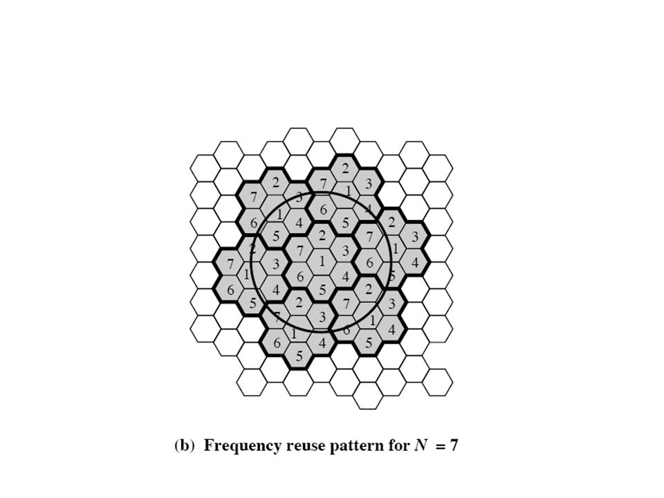
The Cellular Concept Frequency Reuse Pattern for N = 7
Frequency Reuse Factor = 1/7 [Rappa P-59]

Possible Solution (2) Example:
For AMPS (American Advanced Mobile Phone System) Total number of frequencies allotted to the system = K = 395 N = 7 Each cell can have K/ N = 57 frequencies per cell on average

Possible Solution (3) If
D = minimum distance between centers of cells that use same frequency band (called co-channels) R = radius of a cell d = distance b/w cells = 3R Since d = 3R [Rappa P-60]

To Find Nearest Co-Channel
To find nearest co-channel neighbors of a particular cell, one must do the following Move i cells along any chain of hexagons and then Turn 60 degrees counter-clockwise and move j cells. This is illustrated in figure 3.2 for i = 3, and j = 2 (example, N = 19) [Rappa P-60]

19-cell reuse example (N=19)
Fig. 3.2 Figure 3.2 Method of locating co-channel cells in a cellular system. In this example, N = 19 (i.e., I = 3, j = 2). (Adapted from [Oet83] © IEEE.) [Rappa P-60]

Cluster size and Capacity (1)
Let a cellular system has a total of S duplex channels available for use. If each cell is allocated a group of k channels (k < S), and If the S channels are divided among N cells into unique and disjoint channel groups which each have the same number of channels, Total number of available radio channels S = k N [Rappa P-58-60]

CLUSTER: The N cells which collectively use the complete set of available frequencies is called a cluster. Measure of capacity: If a cluster is repeated M times within the system, the total number of duplex channels, C, can be used as a measure of capacity and is given by C = M k N = M S From above, “the capacity of a cellular system”, is directly proportional to the number of times a cluster is replicated in a fixed service area. [Rappa P-58-60]

If the cluster size N is reduced while the cell size is kept constant, more clusters are required to cover a given area, and hence more capacity (a large value of C) is achieved. A larger cluster size causes the ratio b/w the cell radius and the distance b/w co-channel cells (R/D) to decrease, leading to weaker co-channel interference.

Conversely, a small cluster size indicates that co-channel cells are located much closer together. RESULT: Smaller N, gives max C but more interference. The value for N is a function of how much interference a mobile or base station can tolerate while maintaining a sufficient quality of communications. From a design point of view, the smallest possible value of N is desirable in order to maximize capacity over a given coverage area.

Cluster size and Capacity (5) Problem
For an area of 1000 m2, total of 100 duplex channels are allocated. By keeping cell size constant equal to 20 m2, calculate capacity C for following cluster sizes. N = 4 N = 8

Cellular Systems Terms (1)
Frequency Reuse Factor: of a cellular system is given by 1/N, since each cell within a cluster is only assigned 1/N of the total available channels in the system. Cluster Size: The factor N is called the cluster size. Footprint: The actual radio coverage of a cell is known as the footprint and is determined from field measurements or propagation prediction models. [Rappa P-58-60]

Cellular Systems Terms (2)
Base Station (BS) – includes an antenna, a controller, and a number of receivers Mobile telecommunications switching office (MTSO) – connects calls between mobile units Two types of channels available between mobile unit and BS Control channels – used to exchange information having to do with setting up and maintaining calls Traffic channels – carry voice or data connection between users [Rappa P-58-60]

Position of Base Station Transmitters
When using hexagons to model coverage areas, BS transmitters are depicted as either being in the center of the cell (center-excited cells) or on three of the six cell vertices (edge-excited cells). Normally, omni-directional antennas are used in center-excited cells and sectored directional antennas are used in edge-excited cells. Practical considerations do not allow BS to be placed exactly as they appear in the hexagonal layout. Most system designs permit a BS to be positioned up to one-fourth the cell radius away from the ideal location. [Rappa P-58-60]

Example If a total of 33 MHz of bandwidth is allocated to a particular FDD (Frequency Division Duplex, is the first variation of W-CDMA ) cellular telephone system which uses two 25 KHz simplex channels to provide full duplex voice and control channels, compute the number of channels available per cell if a system uses four cell reuse seven cell reuse and Twelve cell reuse If 1 MHz of the allocated spectrum is dedicated to control channels, determine an equitable distribution of control channels and voice channels in each cell for each of the three systems. [Rappa P-61]

Capacity Problem In time, as more customers use the system
traffic may build up so that there are not enough frequency bands (channels) assigned to a cell to handle its calls. It is a Capacity Problem.

Approaches to Cope with Increasing Capacity
Following approaches are used. Adding new channels Frequency borrowing Cell splitting Cell sectoring Microcells A Microcell Zone Concept Femto Cell [Rappa P-86]

Adding new channels Typically, when a system is set up in a region,
Not all of the channels are used, and Growth and expansion can be managed in an orderly fashion by adding new channels.

Frequency borrowing Frequencies are taken from adjacent cells by congested cells Dynamic assignment of frequencies to different cells

Cell splitting (1) Process of subdividing a congested cell into smaller cells (Same concept as of micro-cells), each with its own base station and corresponding reduction in antenna height and transmitter power. It increases the capacity of a cellular system since it increases the number of times that channels are reused. The additional number of channels per unit area

Cell splitting (2) The increased number of cells would  increase the number of clusters over the coverage region,  which in turn would increase the number of channels,  and the capacity, in the coverage area. It allows a system to grow by replacing large cells with smaller cells, while not upsetting the channel allocation scheme required to maintain the minimum co-channel reuse ratio Q between co-channel cells.

Cell splitting (3) A small value of Q means small N  provides large capacity A large value of Q means large N  improves the transmission quality due to a smaller level of co-channel interference. A trade-off must be made b/w these two objectives in actual cellular design

Cell splitting (4) Base stations are placed at the corners of the cells Assume that area served by BS A is saturated with traffic. New BSs are needed to increase the No. of channels in the area and to reduce the area served by single BS BS A has been surrounded by 6 new cells

Cell splitting (5) Cells addition also preserves the frequency reuse plan. Micro cell G has been placed half way b/w two larger stations utilizing the same channel set G. This is also case of other microcells. L/2 L

Cell splitting (6) Distribution of traffic and topographic features is not uniform This presents opportunities of capacity increase Original cell 6.5 to 13 km Cells in areas of high usage can be split into smaller cells 1.5 Km minimum  recommendation Frequent handoff A radius reduction by a factor of F reduces the coverage area and increases the required number of base stations by a factor of F2.

Cell splitting (7) Conclusion: By decreasing the cell radius R, and
keeping the co-channel reuse ratio D/R unchanged, cell splitting increases the number of channels per unit area.

Example Consider Figure 3.9. Assume each base station uses 60 channels, regardless of cell size. If each original cell has a radius of 1 Km and each microcell has a radius of 0.5 Km, find the number of channels contained in a 3 Km by 3 Km square centered around A under the following conditions: without the use of microcells; when the lettered microcells as shown in Figure 3.9 are used, also calculate increase in capacity; and if all the original base stations are replaced by microcells. Assume cells on the edge of the square to be contained within the square.

Solution (a) 5x60 = 300 channels (b) 5+6 = 11 11 x 60 = 660 channels
(c) = 17 channels 17 x 60 = 1020 channels

Cell sectoring Cells are divided into a number of wedge-shaped sectors, Typically three or six sectors per cell Each with their own set of channels Each sector is assigned a separate subset of the cell’s channels Directional antennas are used at the base station to focus on each sector.

Cell sectoring To increase the capacity is
to keep the cell radius unchanged and seek methods to decrease the D/R ratio. Sectoring increases SIR (Signal to Interference Ratio) so that cluster may be reduced. In this approach: First the SIR is improved using directional antennas, Then capacity improvement is achieved by reducing the number of cells in a cluster, Thus increasing the frequency reuse. However, in order to do this successfully, it is necessary to reduce the relative interference without decreasing the transmit power.

Cell sectoring The co-channel interference in a cellular system may be decreased by replacing a single omni directional antenna at the base station by several directional antennas, each radiating within a specified sector. By using directional antennas, a given cell will receive interference and transmit with only a fraction of the available co-channel cells.

Cell sectoring The technique is called sectoring.
for decreasing co-channel interference and thus increasing system performance by using directional antennas is called sectoring.

Sectoring improves S/I
A cell is normally partitioned into three 120 sectors or six 60 Fig. 2.12

Cell sectoring During sectoring Assume
The channels used in a particular cell are broken down into sectored groups and are used only within a particular sector Assume Seven cell reuse 120 sectors

Sectoring improves S/I
Only two cells have sectors with antenna patterns which radiate into the center cell. Compare it with situation of 6 omni directional antennas IV III S/I has been increased from 17dB to 24.2 dB. V II S/I improvement allows the wireless engineer to then decrease the cluster size N in order to improve the frequency reuse and thus system capacity. VI Fig. 2.13 I

Conclusion: Initially co-channels were placed at a distance D due to possible interference. Now we have reduced interference and increased SIR. So we can decrease D and bring co-channels near to each other Thus we decrease N and increase channel capacity.

Cell sectoring Further improvements in S/I:
In practical systems, further improvement in S/I is achieved by down tilting the sector antennas such that the radiation pattern in the vertical (elevation )plane has a notch at the nearest co-channel cell distance

Microcells Microcells are used in As cells become smaller,
city streets congested areas, along highways, and inside large public buildings As cells become smaller, antennas move from the tops of tall buildings or hill  to the top of small buildings or  the sides of large buildings, and finally  to lamp posts, where they form microcells. Decrease in cell size Decrease in radiated power by BS and mobile station

Typical Parameters The average delay spread refers to multipath delay spread that is Same signal follows different paths and There is a time delay between the earliest and latest arrival of the signal at the receiver.

Example Assume a system of 32 cells with a cell radius of 1.6 Km, a total frequency bandwidth that supports 336 traffic channels, and N = 7. If there are 32 total cells, what geographic area is covered? how many channels are there per cell?, and Repeat for a cell radius of 0.8 Km and 128 cells.

The area of hexagon A hexagon of radius 1.6Km has an area 6.65 km2. Total area covered = 6.65 km2 per cell x 32 cells= 213 Km2. No. of channels per cell = 336/7 = 48 channels per cell Total channel capacity = 48 channels per cell x 32 cells = 1536 channels For second fig same 213 Km2 is covered but Channel Capacity = 6144 channels

The Micro Cell Zone Concept

Repeaters for Range Extension
Often a wireless operator needs to provide dedicated coverage for hard-to-reach areas, such as within building, or in valleys or tunnels. Radio re-transmitters, known as repeaters are often used to provide such range extension capabilities. In practice, directional antennas or distributed antenna system (DAS) are connected to the inputs or outputs of repeaters for localized spot coverage, particularly in tunnels or buildings.

[Rappa P-10]

Principal Elements of a Cellular systems
Mobile Telecommunications Switching Office (MTSO) The MSC (Mobile Switching Centre ) and MTSO are one and the same Base Transceiver Station (BTS) Public Telecommunications Switching Network

Base Station (BS/BTS) In the center of each cell there is BS that includes An antenna, A controller, Processes call b/w the mobile unit (MU) and the rest of the network Number of transceivers, For communicating on the channels assigned to that cell.

Cellular System Overview
MTSO

MTSO One MTSO serving multiple BSs
Typically the link b/w MTSO and BS is by wire line, although a wireless link is also possible It connects call b/w MUs It connects public telephone or telecommunication network It assigns the voice channel to each call, performs handoffs and monitors the call for billing information.

Operation of Cellular Systems Channels Type
Two types of channels b/w BS and MU Control channels To exchange information having to do with setting up and maintaining calls and with establishing a relationship b/w MU and nearest BS Traffic channels Carry a voice or data connection b/w users

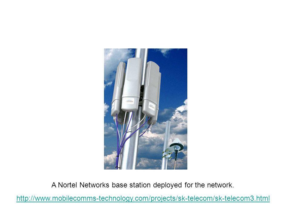
A Nortel Networks base station deployed for the network.

Steps in an MTSO Controlled Call between Mobile Users
Mobile unit initialization Mobile-originated call Paging Call accepted Ongoing call Handoff

Mobile unit initialization
1. MU scans/selects the strongest setup control channel. 2. MU selects the BS 3. Handshake takes place b/w MU and the MTSO through BS 4. Handshake is used to identify the user and to register its location 5. Handshake is repeated periodically to care for handoff

Mobile-originated call
A MU originates a call by sending the number of the called unit on the pre-selected setup channel. MU checks forward channel (from the BS)  transmit on corresponding reverse channel (to BS)

Paging The MTSO sends a paging message to certain BSs depending on the called mobile unit number. Each BS transmits the paging signal on its own assigned setup channel

Call accepted The called MU recognizes its number on the setup channel being monitored and responds to that BS. BS sends the response to MTSO and circuit is setup The MTSO selects an available traffic channel and notifies.

Ongoing call

Handoff While moving from one channel to another
The traffic channel has to change to one assigned to the BS in the new cell. The system makes this change without either interrupting the call or alerting the user.

Additional Functions in an MTSO Controlled Call
Call blocking If all the traffic channels assigned to the nearest BS are busy MU makes a preconfigured number of repeated attempts. After a certain number of failed tries a busy tone is returned to the user. Call termination When one of two users hangs up, the MTSO is informed and … two BSs are released

Additional Functions in an MTSO Controlled Call
Call drop b/c of interference, weak signals BS can not maintain minimum required SNR for a certain period of time The traffic channel to the user is dropped and the MTSO is informed Calls to/from fixed and remote mobile subscriber The MTSO connects to the PSTN. MTSO can set up a connection b/w MU and fixed subscriber. MTSO can connect to a remote MTSO via the telephone network or via dedicated line and set up a connection

[Rappa P-12]

[Rappa P-14]

CAI: Common Air Interface FVC: Forward Voice Channels
RVC: Reverse Voice Channels FCC: Forward Control Channels RCC: Reverse Control Channels MIN: Mobile identification number, which is the subscriber’s telephone number MSC: Mobile Switching Center. It is sometime called a mobile telephone switching office (MTSO) NOTE: Control Channels are also called as Setup channels because they are only involved in setting up a call and moving it to an unused voice channel. [Rappa P-13-15]

Fig. 1.6 Figure 1.6: Timing diagram illustrating how a call to a mobile user initiated by a landline subscriber is established. [Rappa P-16]

Fig. 1.7 Figure 1.7 Timing diagram illustrating how a call initiated by a mobile is established. [Rappa P-17]

Mobile Radio Propagation Effects
Signal strength (SS) Must be strong enough between base station and mobile unit to maintain signal quality at the receiver Must not be so strong as to create too much co-channel interference with channels in another cell using the same frequency band Fading Signal propagation effects may disrupt the signal and cause errors

Mobile Radio Propagation Effects
In designing a cellular layout The desired maximum transmit power level at the BS and the MU The typical height of the MU antenna The available height of the BS antenna These factors determine the size of Cell

Channel (Path Loss) Model
Propagation effects are dynamic and difficult to predict Find a model based on empirical data One of the most famous widely used models was developed by Okumura et al.

Channel (Path Loss) Model
Okumura Model was subsequently refined by Hata. Hata’s Model  Empirical formulation Takes into account a variety of environments and conditions. Models are applied to  a given environment to  develop guidelines for  Cell Size

On Whiteboard

Example For a carrier frequency of 900 MHz, ht = 40m, hr = 5m, and d = 10 Km. Estimate the path loss for a medium size city. A(hr) = 8.95 dB LdB = dB

Handoff/ Handover Both Handoff and Handover have same meaning.
The term Handoff is used in U.S cellular standards document ITU documents use the term Handover.

Handoff What is? It is the procedure for
changing the assignment of a MU from one BS to another as the MU. Handled in different ways in different systems. Involves a number of factors

Handoff Initiation May be Network Initiated
Decision is made solely by the network measurements of received signals from the MU. Mobile Assisted Handoff (MAHO) MU provides feedback to the network concerning signals received at the MU.

Handoff Performance Metrics
Call blocking probability Probability of a new call being blocked, due to heavy load on the BS traffic capacity. MU is handed off based not on signal quality but on traffic capacity. Call dropping probability probability that a call is terminated due to a handoff

Call completion probability Probability that an admitted call is not dropped before it terminates Probability of unsuccessful handoff Probability that a handoff is executed while the reception conditions are inadequate Example: Time lapse Handoff blocking probability Probability that a handoff cannot be successfully completed Example: Other BS busy

Handoff probability Probability that a handoff occurs before call termination Rate of handoff Number of handoffs per unit time Interruption duration Duration of time during a handoff in which a mobile is not connected to either base station Handoff delay Distance the mobile moves from the point at which the handoff should occur to the point at which it does occur

Handoff Decision Principal parameter is SS. SS is measured from the MU
BS averages signal over a moving window of time to remove the rapid fluctuations due to multi-path effects.

Handoff strategies These strategies are used to Determine Instant of Handoff Relative SS Relative SS with threshold Relative SS with hysteresis Relative SS with hysteresis and threshold Prediction techniques

Handoff decision as a function of handoff scheme

Relative SS The MU is handed off from BS A to BS B when the Signal Strength (SS) at B first exceeds that at A. At L1, SS is adequate but declining there is hand off. b/c SS fluctuates due to multi-path effects, even with power averaging  SS again may increase  handoff back to A. Problem: This may result in ping-pong effect.

Choosing Threshold If high threshold Th1 is used  system performs like Relative SS scheme. If low threshold Th3 is used,  quite low as compared to the crossover SS (at L1) before handoff. MU will move far in into the new cell This reduces the quality of the communication link It may result in a dropped call. A threshold should not be used alone b/c its effectiveness depends on prior knowledge of the crossover SS b/w current and candidate BSs.

Relative SS with hysteresis (1)
Handoff occurs only if the new BS is sufficiently stronger  by a margin of H. Look at graph, After crossover point PB > PA At L3, PB - PA = H Handoff occurs at L3.

Relative SS with hysteresis (2)
This scheme prevents the ping-pong effect Handoff mechanism has two states While the MU is assigned to BS A, the mechanism will generate a handoff when the relative SS reaches or exceeds the H. Once the MU is assigned to B, it remains so until the relative SS strength falls below –H, at which point is handed back to A. Disadvantage: First handoff may still be unnecessary if BS A still has sufficient SS.

Relative SS with hysteresis and Threshold
Handoff occurs only if The current signal level drops below a threshold, and The target BS is stronger than the current one by a hysteresis margin H. In our example, handoff occurs at L3. if the threshold is either Th1 or Th2 and at L4 if the threshold is at Th3.

Prediction Technique The handoff decision is based on
the expected future value of the received SS.

Handoff priority Many handoff strategies prioritize handoff requests over call initiation requests when allocating unused channels in a cell site. Handoff must be performed successfully and infrequently as possible. Handoff must be imperceptible to the users. [Rappa P-62-67]

Proper signal level (1) Signal Level Specification for Handoff
Once a particular signal level is specified as the minimum usable signal for acceptable voice quality at the BS receiver Normally taken as b/w -90 dBm and -100 dBm a slightly stronger level is used as a threshold at which a handoff is made. [Rappa P-62-67]

 = Pr handoff – P r minimum usable
Proper signal level (2) The margin, given by  = Pr handoff – P r minimum usable  can not be too large b/c unnecessary handoffs which burden the MTSO may occur  can not be too small There may be insufficient time to complete a handoff before a call is lost due to weak signal conditions. [Rappa P-62-67]

Example [Rappa P-62-67]

Possible reasons of NO handoff
When there is an excessive delay by the MSC (MTSO) in assigning a handoff or when the threshold  is set too small for the handoff time in the system. Excessive delays may occur during high traffic conditions due to computational loading at the MSC or due to the fact that no channels are available on any of the nearby BSs [Rappa P-62-67]

Dwell time The time over which a call may be maintained within a cell, without handoff, is called the dwell time. The dwell time, of a particular user is governed by a number of factors, including Propagation Interference Distance between the subscriber and the BS Other time varying effects.

Implementations In first generation cellular systems, SS measurement are made by the BSs and supervised by the MSC. In today’s second generation systems, handoff decisions are mobile assisted (MAHO) [Rappa P-62-67]

First Generation - Analog
Each BS constantly monitors the SS of all of its reverse voice channels (RVC) to determine the relative location of each MU with respect to BS tower. Locator Receiver (LR): in addition to measuring the RSSI of calls in progress within the cell, a spare receiver in each BS, called LR is used to scan and determine SS of MUs which are in neighbouring cells. LR is controlled by MSC Based on the LR SS info from BS, the MSC decides handoff.

Second Generation Each MU measures the received power from surrounding BS and continually reports the results of these measurements to the serving BS. A handoff is initiated when the power received from the BS of a neighboring cell begins to exceed the power received from the current base station by a certain level or for a certain period of time.

MAHO The MAHO method enables the call to be handed over b/w BSs at a much faster rate than in first generation analog systems Since the handoff measurements are made by each MU and The MSC no longer constantly monitors SS MAHO is particularly suited for microcellular environments where handoffs are more frequent.

Intersystem handoff If a mobile moves from one cellular system to a different cellular system controlled by a different MSC  Intersystem handoff becomes necessary Many issues Local call may become a long distance call Compatibility between two MSCs before handoff

Managing Handoff (1) Different systems have different policies and methods for managing handoff requests Some systems handle handoff request in the same way they handle originating calls. In such systems, the probability that a handoff request will not be served by a new BS is equal to the blocking probability of incoming calls. However, from the users point of view, having a call abruptly terminated while in the middle of a conversation is more annoying than being blocked occasionally on a new call attempt.

Managing Handoff (2) To improve the QoS as perceived by the users, various methods have been devised to prioritize handoff requests over call initiation requests when allocating voice channels. Prioritizing Handoffs Guard Channel Concepts Queuing of handoff requests Practical Handoff Considerations Umbrella Cell Approach  solution to a problem Cell Dragging  is a problem

Guard Channel Concepts
Channel Reservation: Fraction of total available channels in a cell is reserved exclusively for handoff requests Disadvantage: Reduces the total carried traffic (CT)  as fewer channels are allocated for originating calls. Possible Solution: Use of dynamic channel assignment strategies  Minimize the No. of required guard channels by efficient demand based allocation Provides efficient spectrum utilization

Queuing of handoff requests (1)
Criteria: There must be finite time interval b/w the time the RSS drops below the handoff threshold and the time the call is terminated due to insufficient signal level.

Queuing of handoff requests (2)
It is one of the methods to decrease the probability of forced termination (PFT) of a call due to lack of available channels. There is a tradeoff b/w CT & PFT Queuing does not guarantee zero probability of forced termination Since large delays will cause the RSS to drop below the minimum required level to maintain communication and hence lead to forced termination

Practical Handoff Considerations
During a call High speed vehicles need more handoff Pedestrians may never need a handoff For micro-cells MSC become burdened if high speed users are constantly being passed b/w very small cells. Problem Handling of high speed and low speed traffic simultaneously  while minimizing the handoff intervention from MSC Solution: Umbrella Cell approach

Umbrella Cell approach
“Large” and “Small” cells are Provided by using different antenna heights (often on the same building and towers) and different power levels and Co-located at a single location Provides large area coverage to high speed users while small area coverage to users traveling at low speeds.

Umbrella Cell Approach

This approach ensures that the number of handoffs is minimized for high speed users and provides additional micro-cell channels for pedestrian users.

Scenario: A driver in a high speed car is attending a call on mobile telephone, present in a large cell enters in a micro cell. Discuss the responsibility of BS/MSC

The speed of each user may be estimated by the BS or MSC by Evaluating how rapidly the short-term average signal strength on the RVC changes over time, OR More sophisticated algorithms may be used o evaluate and partition users. If a high speed user in the large umbrella cell is approaching the BS and its velocity is rapidly decreasing, the BS may decide to hand the user into the co-located micro-cell, without MSC intervention.

Cell Dragging (1) Problem of Cell Dragging
It occurs in an urban environment when there is a LOS radio path b/w the subscriber and the BS. As the user travels away from the BS at very slow speed, the average SS does not decay rapidly. Even when the user has traveled well beyond the designed range of the cell, the RSS at the BS may be above the handoff threshold, Thus a handoff may not be made

Cell Dragging (2) This creates a potential interference and traffic management problem Since the user has meanwhile traveled deep within a neighboring cell. Solution: Handoff threshold and radio coverage parameters must be adjusted carefully.

Handoff Time First generation- Analog Cellular Systems 10 Seconds GSM
Requires that the value of  be on the order of 6 dB to 12 dB GSM MAHO 1or 2 Seconds, after decision is made  is usually on the order of 0 dB to 6 dB Advantage: Faster handoff  greater range of options for handling high speed and low speed users

Recent Trends in handoff
Two types Hard handoff Channelized wireless systems that assign different radio channels during a handoff Soft handoff It is the ability to select b/w the instantaneous RSS from a variety of BS.

Soft handoff Spread Spectrum mobiles (Code Division Multiple Access, CDMA) share the same channel in every cell. By simultaneously evaluating the RSS from a single subscriber at several neighboring BSs, The MSC may actually decide which version of the user’s signal is the best at any moment in time. This technique exploits macroscopic space diversity provided by the different physical locations of the BS.

Power Control Design issues making it desirable to include dynamic power control in a cellular system Received power must be sufficiently above the background noise for effective communication Desirable to minimize power in the transmitted signal from the mobile Reduce co-channel interference, alleviate health concerns, save battery power In Spread Spectrum systems using CDMA, it’s desirable to equalize the received power level from all mobile units at the BS

Types of Power Control (1)
1. Closed-loop power control Adjusts signal strength in reverse channel (MU to BS) based on some metric of performance in that reverse channel, such as Received signal power level Received signal-to-noise ratio, or Received bit error rate BS makes power adjustment decision and communicates to MU on control channel

Closed loop power control is also used to adjust power in the forward channel. In this case MU provides information about received signal quality to the BS, which then adjusts transmitted power. GSM standard  a TDMA standard defines, according to power output Eight classes of BS channels and Five classes of MU

GSM Transmitter Classes
Adjustments in both directions are made using closed loop power control

2. Open-loop power control Depends solely on mobile unit with no feedback from BS  used in some spread spectrum systems (SSS). In SSS, the BS continuously transmits an unmodulated signal known as a pilot. The pilot allows MU to acquire the timing of the forward (BS to mobile) CDMA channel.

It can also be used for power control. The MU monitors the RSS of the pilot and sets the transmitted power in the reverse (mobile to BS) channel inversely proportional to it. Assumption: Forward and Reverse link RSS are correlated.

Not as accurate as closed-loop, but can react quicker to fluctuations in signal strength E.g when MU emerges from behind a large building. This fast action is required in the reverse link of a CDMA systems where the sudden increase in RSS at the BS may suppress all other signals.

Trunking Theory (1)

Trunking Theory (2) Trunked Radio Systems
share a small pool of frequencies among a large number of users The benefit of this technology to the agencies is that many more channels are available for specialized traffic than there are frequencies. Example, the Fort Worth trunked system has only 20 frequencies, but services over 400 channels.

Trunking Theory (3) Trunking is the aggregation of multiple user circuits into a single channel. The aggregation is achieved using some form of multiplexing. Trunking theory was developed by Agner Krarup Erlang, Erlang based his studies of the statistical nature of the arrival and the length of calls. The Erlang B formula allows for the calculation of the number of circuits required in a trunk based on the Grade of Service (GoS) and the amount of traffic in Erlangs the trunk needs cater for.

Key Definitions for Trunked Radio
Fig. 2.6

Traffic Engineering The Danish mathematician Agner Krarup Erlang is the founder of teletraffic engineering. Ideally, available channels would equal number of subscribers active at one time In practice, not feasible to have capacity handle all possible load For N simultaneous user capacity and L subscribers L < N – nonblocking system L > N – blocking system

Blocking System Performance Questions
Probability that call request is blocked? OR What capacity is needed to achieve a certain upper bound on probability of blocking? If blocked calls are queued, what is the average delay? OR What capacity is needed to achieve a certain average delay?

Traffic Intensity (1) The basic measure of traffic intensity is A.
It is measured in a dimensionless unit, the erlang  = mean rate of calls attempted per unit time h = mean holding time per successful call A = average number of calls arriving during average holding period, for normalized 

Traffic Intensity (2) Cell as a Multiserver Queuing System:
No. of servers equal to channel capacity, N. The average service time at a server is h. A basic relationship in a multiserver queue is h = N Where  is server utilization, or the fraction of time that a server is busy. Note: A = N, is considered as a measure of the average number of channels required.

Traffic Intensity (3) Example:
What should be capacity of the cell to meet average demand, for average calling rate of 20 calls per minute and average holding time 3 minutes? To meet the fluctuations, what do you suggest about the capacity of the cell?

Traffic Intensity (4) Example:
A cell having 10 channels is busy over a period of one hour as shown in the figure. Calculate mean number of channels busy for this time.

Traffic Modeling (1) Upper limit of traffic intensity?
ITU-T  “mean busy hour traffic” Average of the busy-hour-traffic on the 30 busiest day A is measure of busy-hour-traffic A is input to traffic model Traffic model answers the questions posed.

See detail on next slide
Traffic Modeling (2) Two key factors/elements that determines the nature of traffic model The manner in which blocked calls are handled Then number of traffic sources. See detail on next slide

For Cellular systems, the LCC model is generally used  most accurate
Traffic Modeling (3) Manner in which blocked calls are handled Lost calls delayed (LCD) – blocked calls put in a queue awaiting a free channel Blocked calls rejected and dropped Lost calls cleared (LCC) – user waits before another attempt Lost calls held (LCH) – user repeatedly attempts calling For Cellular systems, the LCC model is generally used  most accurate Number of traffic sources Whether number of users is assumed to be finite or infinite

Traffic Modeling (4) Erlang B
Infinite Source, LCC Model: The key parameter is the probability of loss, or grade of Service (GoS). GoS = 0.01 means that, during a busy hour, the probability that an attempted call is blocked is 0.01 Values in the range 0.01 to are generally considered quite good.

Traffic Modeling (5) Erlang B
Following equation is known as Erlang B. P = Probability of blocking (grade of service) A = Offered traffic, erlangs N = Number of servers

Traffic Modeling (6)

Illustrations of these points on next slides
Traffic Modeling (7) Two important points can be deduced from the table: A larger-capacity system is more efficient than a smaller-capacity one for a given grade of service. A larger-capacity system is more susceptible (open) to an increase in traffic. Illustrations of these points on next slides

Traffic Modeling (8) Illustrations: First point Consider two cells,
each with a capacity of 10 channels Joint capacity of 20 channels Look in column GoS=0.002 Traffic intensity for 10 channels = 3.43 Traffic intensity for 20 channels = 6.86 For a single cell of 20 channels Traffic intensity = 10.07

Traffic Modeling (9) Second point
Consider a single cell of 10 channels, Look in column GoS=0.002 Traffic intensity/ Load = 3.43 Erlangs 30% increase in the traffic reduces the GoS to 0.01 Consider a single cell of 70 channels, Traffic intensity/ Load = 51.0 Erlangs Only 10% increase in the traffic reduces the GoS from to 0.01

Traffic Modeling (10) Effect of Handoff .

Cellular Wireless Networks

Similar presentations

Presentation on theme: "Cellular Wireless Networks"— Presentation transcript:

Similar presentations

About project

Feedback

Log in

Auth with social network:

Cellular Wireless Networks

Similar presentations

Presentation on theme: "Cellular Wireless Networks"— Presentation transcript:

Similar presentations

About project

Feedback