1. Chapter 6 The 2k Factorial Design

2. 6.1 Introduction
The special cases of the general factorial design (Chapter 5)
k factors and each factor has only two levels
Levels:
quantitative (temperature, pressure,…), or qualitative (machine, operator,…)
High and low
Each replicate has 2    2 = 2k observations

3. Assumptions: (1) the factor is fixed, (2) the design is completely randomized and (3) the usual normality assumptions are satisfied
Wildly used in factor screening experiments

4. 6.2 The 22 Factorial Design
Two factors, A and B, and each factor has two levels, low and high.
Example: the concentration of reactant v.s. the amount of the catalyst (Page 219)

5. “-” And “+” denote the low and high levels of a factor, respectively
Low and high are arbitrary terms
Geometrically, the four runs form the corners of a square
Factors can be quantitative or qualitative, although their treatment in the final model will be different

6. Average effect of a factor = the change in response produced by a change in the level of that factor averaged over the levels if the other factors.
(1), a, b and ab: the total of n replicates taken at the treatment combination.
The main effects:

7. The interaction effect:
In that example, A = 8.33, B = and AB = 1.67
Analysis of Variance
The total effects:

8. Sum of squares:

9. Response:. Conversion. ANOVA for Selected Factorial Model
Response: Conversion ANOVA for Selected Factorial Model Analysis of variance table [Partial sum of squares]
Sum of Mean F Source Squares DF Square Value Prob > F Model A < B AB Pure Error Cor Total
Std. Dev R-Squared Mean Adj R-Squared C.V Pred R-Squared
PRESS Adeq Precision
The F-test for the “model” source is testing the significance of the overall model; that is, is either A, B, or AB or some combination of these effects important?

10. Table of plus and minus signs:
(1) + – a b ab

11. The regression model:
x1 and x2 are coded variables that represent the two factors, i.e. x1 (or x2) only take values on –1 and 1.
Use least square method to get the estimations of the coefficients
For that example,
Model adequacy: residuals (Pages 224~225) and normal probability plot (Figure 6.2)

12. Response surface plot:
Figure 6.3

13. 6.3 The 23 Design
Three factors, A, B and C, and each factor has two levels. (Figure 6.4 (a))
Design matrix (Figure 6.4 (b))
(1), a, b, ab, c, ac, bc, abc
7 degree of freedom: main effect = 1, and interaction = 1

15. Estimate main effect:
Estimate two-factor interaction: the difference between the average A effects at the two levels of B

16. Three-factor interaction:
Contrast: Table 6.3
Equal number of plus and minus
The inner product of any two columns = 0
I is an identity element
The product of any two columns yields another column
Orthogonal design
Sum of squares: SS = (Contrast)2/8n

17. Table of – and + Signs for the 23 Factorial Design (pg. 231)
Factorial Effect
Treatment
Combination I A B AB C AC BC
ABC
(1) + – a b ab c ac bc
abc
Contrast 24 18 6 14 2 4
Effect
3.00
2.25
0.75
1.75
0.25
0.50

18. Example 6.1
A = carbonation, B = pressure, C = speed, y = fill deviation

19. Estimation of Factor Effects
Term Effect SumSqr % Contribution Model Intercept Error A Error B Error C Error AB Error AC Error BC Error ABC Error LOF 0 Error P Error
Lenth's ME Lenth's SME

20. ANOVA Summary – Full Model
Response: Fill-deviation ANOVA for Selected Factorial Model Analysis of variance table [Partial sum of squares]
Sum of Mean F Source Squares DF Square Value Prob > F Model A < B C AB AC BC ABC Pure Error Cor Total
Std. Dev R-Squared Mean Adj R-Squared C.V Pred R-Squared
PRESS Adeq Precision

21. The regression model and response surface: The regression model:
Response surface and contour plot (Figure 6.7)
Coefficient Standard 95% CI 95% CI Factor Estimate DF Error Low High Intercept A-Carbonation B-Pressure C-Speed AB

22. Contour & Response Surface Plots – Speed at the High Level

23. Refine Model – Remove Nonsignificant Factors
Response: Fill-deviation ANOVA for Selected Factorial Model Analysis of variance table [Partial sum of squares]
Sum of Mean F Source Squares DF Square Value Prob > F Model < A < B C AB Residual LOF Pure E C Total
Std. Dev R-Squared Mean Adj R-Squared C.V Pred R-Squared
PRESS Adeq Precision

24. 6.4 The General 2k Design k factors and each factor has two levels
Interactions
The standard order for a 24 design: (1), a, b, ab, c, ac, bc, abc, d, ad, bd, abd, cd, acd, bcd, abcd

25. The general approach for the statistical analysis:
Estimate factor effects
Form initial model (full model)
Perform analysis of variance (Table 6.9)
Refine the model
Analyze residual
Interpret results

26. 6.5 A Single Replicate of the 2k Design
These are 2k factorial designs with one observation at each corner of the “cube”
An unreplicated 2k factorial design is also sometimes called a “single replicate” of the 2k
If the factors are spaced too closely, it increases the chances that the noise will overwhelm the signal in the data

27. Lack of replication causes potential problems in statistical testing
Replication admits an estimate of “pure error” (a better phrase is an internal estimate of error)
With no replication, fitting the full model results in zero degrees of freedom for error
Potential solutions to this problem
Pooling high-order interactions to estimate error (sparsity of effects principle)
Normal probability plotting of effects (Daniels, 1959)

28. Example 6.2 (A single replicate of the 24 design)
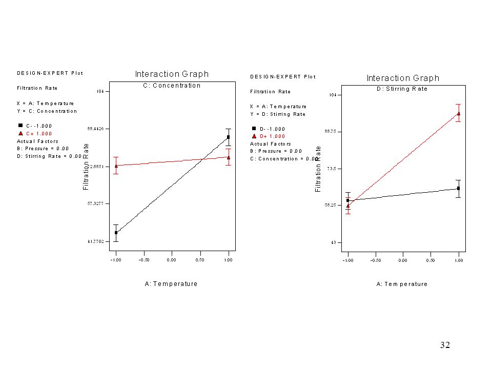
A 24 factorial was used to investigate the effects of four factors on the filtration rate of a resin
The factors are A = temperature, B = pressure, C = concentration of formaldehyde, D= stirring rate

30. Estimates of the effects
Term Effect SumSqr % Contribution Model Intercept Error A Error B Error C Error D Error AB Error AC Error AD Error BC Error BD Error CD Error ABC Error ABD Error ACD Error BCD Error ABCD
Lenth's ME Lenth's SME

31. The normal probability plot of the effects

33. B is not significant and all interactions involving B are negligible
Design projection: 24 design => 23 design in A,C and D
ANOVA table (Table 6.13)

34. Response:. Filtration Rate. ANOVA for Selected Factorial Model
Response: Filtration Rate ANOVA for Selected Factorial Model Analysis of variance table [Partial sum of squares]
Sum of Mean F Source Squares DF Square Value Prob >F Model < A < C D < AC < AD < Residual Cor Total
Std. Dev R-Squared Mean Adj R-Squared C.V Pred R-Squared
PRESS Adeq Precision

35. The regression model: Residual Analysis (P. 251)
Response surface (P. 252)
Final Equation in Terms of Coded Factors:
Filtration Rate = * Temperature * Concentration * Stirring Rate * Temperature * Concentration * Temperature * Stirring Rate

37. Half-normal plot: the absolute value of the effect estimates against the cumulative normal probabilities.

38. Example 6.3 (Data transformation in a Factorial Design)
A = drill load, B = flow, C = speed, D = type of mud, y = advance rate of the drill

39. The normal probability plot of the effect estimates

40. Residual analysis

41. The residual plots indicate that there are problems with the equality of variance assumption
The usual approach to this problem is to employ a transformation on the response
In this example,

42. Three main effects are large
No indication of large interaction effects
What happened to the interactions?

43. Response:. adv. _rate. Transform: Natural log. Constant: 0. 000
Response: adv._rate Transform: Natural log Constant: ANOVA for Selected Factorial Model
Analysis of variance table [Partial sum of squares] Sum of Mean F Source Squares DF Square Value Prob > F Model < B < C < D Residual Cor Total
Std. Dev R-Squared Mean Adj R-Squared C.V Pred R-Squared
PRESS Adeq Precision

44. Following Log transformation
Final Equation in Terms of Coded Factors:
Ln(adv._rate) = * B * C * D

46. Example 6.4:
Two factors (A and D) affect the mean number of defects
A third factor (B) affects variability
Residual plots were useful in identifying the dispersion effect
The magnitude of the dispersion effects:
When variance of positive and negative are equal, this statistic has an approximate normal distribution

47. 6.6 The Addition of Center Points to the 2k Design
Based on the idea of replicating some of the runs in a factorial design
Runs at the center provide an estimate of error and allow the experimenter to distinguish between two possible models:

48. The hypotheses are:
This sum of squares has a single degree of freedom

49. Example 6.6 Usually between 3 and 6 center points will work well
Design-Expert provides the analysis, including the F-test for pure quadratic curvature

50. Response:. yield. ANOVA for Selected Factorial Model
Response: yield ANOVA for Selected Factorial Model Analysis of variance table [Partial sum of squares]
Sum of Mean F Source Squares DF Square Value Prob > F Model A B AB 2.500E E Curvature 2.722E E Pure Error Cor Total
Std. Dev R-Squared Mean Adj R-Squared
C.V Pred R-Squared N/A
PRESS N/A Adeq Precision

51. If curvature is significant, augment the design with axial runs to create a central composite design. The CCD is a very effective design for fitting a second-order response surface model