1. Pushing Astrometry to the Limit Richard Berry

2. Barnard’s Star Location: Ophiuchus Location: Ophiuchus Coordinates: 17 h 57 m 48.5 +4º41’36”(J2000) Coordinates: 17 h 57 m 48.5 +4º41’36”(J2000) Apparent Magnitude: V = 9.54 (variable) Apparent Magnitude: V = 9.54 (variable) Spectral Class: M5V (red dwarf) Spectral Class: M5V (red dwarf) Proper Motion: 10.33777 arc-seconds/year Proper Motion: 10.33777 arc-seconds/year Parallax: 0.5454 arc-seconds Parallax: 0.5454 arc-seconds Distance: 5.980±0.003 light-years Distance: 5.980±0.003 light-years Radial Velocity: –110.6 km/second Radial Velocity: –110.6 km/second Rotation Period: 130.4 days Rotation Period: 130.4 days

3. Proper Motion 90 km/s -111 km/s -141 km/s 10.34 arc-seconds/year Closest in ~12,000 AD 5.980 light-years

4. N S EW Barnard’s “Flying Star”

5. Astrometry with CCDs Requirements: Requirements: –An image showing the object to be measured. –At least three reference stars in the image. –An astrometric catalog of reference stars (UCAC2). –Approximate coordinates for the image. –Software written for doing astrometry. Data also needed: Data also needed: –Observer’s latitude, longitude, and time zone. –The dates and times images were made.

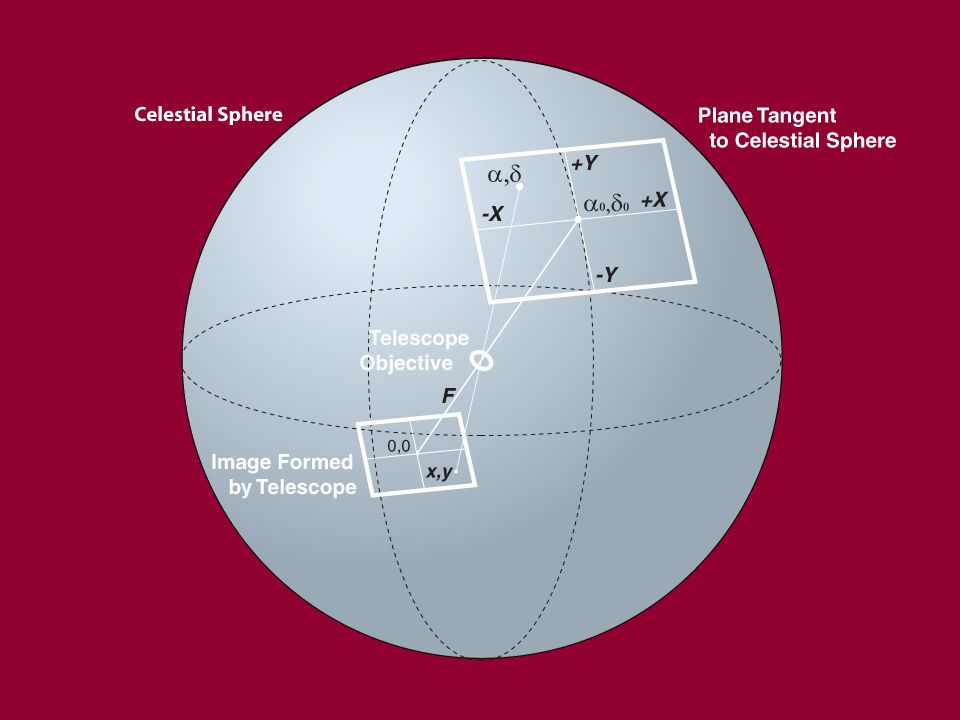
7. (α,δ)  (X,Y) When you shoot an image, you’re mapping the celestial spherical onto a plane surface. When you shoot an image, you’re mapping the celestial spherical onto a plane surface. This occurs for all the stars in the image, both the target stars and the reference stars. This occurs for all the stars in the image, both the target stars and the reference stars. The standard (X,Y) coordinates of a star at (α,δ) for an image centered on (α 0,δ 0 ) are: The standard (X,Y) coordinates of a star at (α,δ) for an image centered on (α 0,δ 0 ) are: X = (cosδ sin(α-α 0 ))/d Y = (sinδ 0 cosδ cos(α-α 0 )- cosδ 0 sinδ)/d where d = cosδ 0 cosδ cos(α-α 0 )+sinδ 0 sinδ.

8. This represents a plane tangent to the sky. Each star at some (α,δ) has standard coordinates (X,Y).

10. This represents an image captured by a CCD camera. Each star in the image has a location (x, y).

11. The CCD Image Known properties of the image: Known properties of the image: –Approximate center coordinates: (α 0,δ 0 ). –Approximate focal length of telescope = F. Unknown properties of the image: Unknown properties of the image: –Offset distance in x axis: x offset. –Offset distance in y axis: y offset. –Rotation relative to north-at-top = ρ.

12. The image is offset, rotated, and scaled with respect to standard coordinates.

13. Reference stars Astrometric catalogs are lists of stars with accurately measured (α,δ) coordinates. Astrometric catalogs are lists of stars with accurately measured (α,δ) coordinates. –Guide Star Catalog (GSC) –USNO A2.0 –UCAC2 or UCAC3 Astrometric catalogs often list millions of stars. Astrometric catalogs often list millions of stars. We use the reference stars in the image to link image coordinates to standard coordinates. We use the reference stars in the image to link image coordinates to standard coordinates. A minimum of three reference stars are needed. A minimum of three reference stars are needed.

14. By offsetting, rotating, and scaling standard coordinates, we can link each reference star with its counterpart in the image. Ref Star 1  Ref Star 3  Ref Star 2 

15. What do we know? We know: We know: –Three or more reference stars in the image. –Approximate coordinates of image center (α 0,δ 0 ). –For each reference star, its (α,δ) coordinates. –For each reference, its standard coordinates (X,Y). –For each reference, we measure (x,y) from the image. –For target object(s), we measure (x,y) coordinates. We want: We want: –The (α,δ) coordinates of the target object.

16. (x,y)  (X,Y) To offset, rotate, and scale coordinates: To offset, rotate, and scale coordinates: –X = x cosρ/F + y sinρ/F + x offset /F –Y = x sinρ/F + y cosρ/F + y offset /F But we do not know ρ, F, or the offsets. But we do not know ρ, F, or the offsets. However, for each reference star, we know: However, for each reference star, we know: –(X,Y) standard coordinates, and –(x,y) image coordinates.

17. Linking the Coordinates Suppose we have three reference stars. Suppose we have three reference stars. For each star, we know (x,y) and (X,Y). For each star, we know (x,y) and (X,Y). –X 1 = ax 1 + by 1 + c and Y 1 = dx 1 + dy 1 + f –X 2 = ax 2 + by 2 + c and Y 2 = dx 2 + dy 2 + f –X 3 = ax 3 + by 3 + c and Y 3 = dx 3 + dy 3 + f. Three equations, three unknowns  solvable. Three equations, three unknowns  solvable. In the X axis, we solve for a, b, and c. In the X axis, we solve for a, b, and c. In the Y axis, we solve for d, e, and f. In the Y axis, we solve for d, e, and f.

18. Computing Target Coordinates From reference stars, we find a, b, c, d, e, and f. From reference stars, we find a, b, c, d, e, and f. The standard coordinates of the target are: The standard coordinates of the target are: –X target = ax target + by target + c, and –Y target = dx target + ey target + f Given (X,Y) for the target, it’s (α,δ) is: Given (X,Y) for the target, it’s (α,δ) is: –δ = arcsin((sinδ 0 +Ycosδ 0 )/(  1+X 2 +Y 2 )), and –α = α 0 + arctan(X/(cosδ 0 +Ysinδ 0 )). Ta-da! Ta-da!

19. Parallax: Mission Impossible Difficult Goals: Goals: –Repeatedly measure  and  for a year. –Attain accuracy ~1% the expected parallax. –Reduce and analyze the measurements. Problems to overcome: Problems to overcome: –Differential refraction displacing stars. –Instrumental effects of all kinds. –Under- and over-exposure effects. –Errors and proper motion in reference stars.

20. Shooting Images When to shoot When to shoot –If possible, near the meridian. –If possible, on nights with good seeing. –If possible, once a week, more often when star 90º from Sun. Filters Filters –To minimize differential refraction, use V or R. Reference stars Reference stars –Select reference stars with low proper motion. –Set exposure time for high signal-to-noise ratio. Target star Target star –Do not allow image to reach saturation. How many images? How many images? –Shoot as many as practical to shoot and reduce.

21. Extracting Coordinates In AIP4Win, semi-automated process In AIP4Win, semi-automated process –Observer must exercise oversight. –Check/verify all ingoing parameters. –Select an optimum set of reference stars. –Supervise extraction and processing. –Inspect reported data. –Check discrepancies and anomalies.

22. N S EW

23. N S EW Define a set of reference stars…

24. Getting started…

25. Observer Properties…

26. Instrument Properties…

27. Image Selection…

28. Set the aperture and annulus…

29. Select the target object…

30. Select the reference stars…

31. Select a guide star and let ‘er rip…

32. Check then save the astrometry report…

33. Examination Copy data to Excel (or other spreadsheet) Copy data to Excel (or other spreadsheet) –Importing is easy when text data is delimited. –Check the “canaries”: focal length, position angle. –Check the residuals in  and . –Compute (  ) mean and standard deviation. –Plot individual and mean positions. Long term Long term –Plot the individual and mean positions for all nights. –Apply lessons learned to future observations.

34. Importing a text file…

35. Astrometry data imported into Excel…

36. Check the “canaries”…

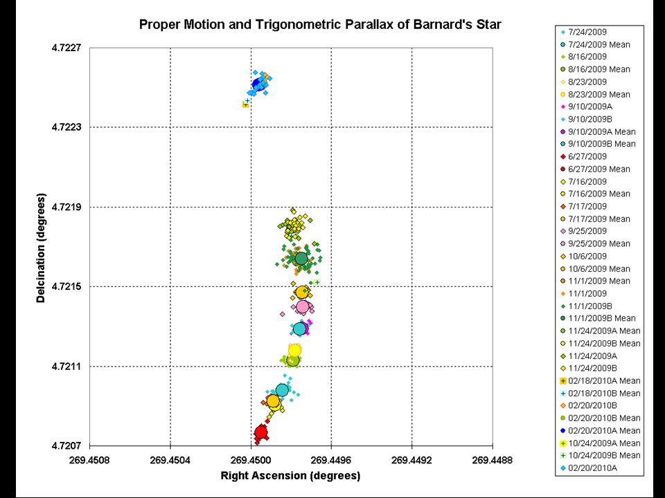
37. One night’s results from 40 images… 0.25 arcseconds

39. The Next Steps… Model based on five parameters: Model based on five parameters: –Initial RA (J 2000.0) –Initial DEC (J 2000.0) –PM in RA –PM in DEC –Parallax –These known from Hipparcos Mission Compute parameters from observations Compute parameters from observations –Solve matrix of observed (RA,DEC). –Least-squares method for best fit to observations.

40. Computing a star’s position…  now =  J2000.0 +  PM (Y now –2000) +  P   now =  J2000.0 +  PM (Y now –2000) +  P  (  ) now = current coordinates (  ) now = current coordinates (  ) J2000.0 = coordinates in J2000.0 (  ) J2000.0 = coordinates in J2000.0  PM = annual proper motion in RA  PM = annual proper motion in RA  PM = annual proper motion in Dec  PM = annual proper motion in Dec  = parallax of the star  = parallax of the star P  = parallax factor in  for time Y now P  = parallax factor in  for time Y now P  = parallax factor in  for time Y now P  = parallax factor in  for time Y now

41. Observed positions…

42. Observed and computed positions…

43. Parallax only…

44. Proper motion only…

45. Motion over 3 years…

46. Small-Telescope Astrometry With a focal length ~1,000mm. With a focal length ~1,000mm. Ordinary CCD with 6.4 micron pixels. Ordinary CCD with 6.4 micron pixels. Selected set of reference stars. Selected set of reference stars. Observation with multiple images. Observation with multiple images. Using optimized exposure time. Using optimized exposure time. Routinely achieves 0.020 arcsecond accuracy. Routinely achieves 0.020 arcsecond accuracy. Sometimes achieves 0.010 arcsecond accuracy. Sometimes achieves 0.010 arcsecond accuracy.

47. Resources

49. Pushing Astrometry to the Limit Richard Berry