2. Johann Radon Institute for Computational and Applied Mathematics Linz, Österreich 15. März 2004

3. Johann Radon Institute for Computational and Applied Mathematics Linz, Österreich 15. März 2004

4. trummer@sfu.catrummer@sfu.ca www.math.sfu.ca/~mrt Richard Baltensperger Université Fribourg Manfred Trummer Pacific Institute for the Mathematical Sciences & Simon Fraser University Johann Radon Institute for Computational and Applied Mathematics Linz, Österreich 15. März 2004

5. Pacific Institute for the Mathematical Sciences www.pims.math.ca

6. Simon Fraser University

7. Banff International Research Station PIMS – MSRI collaboration (with MITACS) 5-day workshops 2-day workshops Focused Research Research In Teams www.pims.math.ca/birs

8. Round-off Errors 1991 – a patriot missile battery in Dhahran, Saudi Arabia, fails to intercept Iraqi missile resulting in 28 fatalities. Problem traced back to accumulation of round-off error in computer arithmetic. 1991 – a patriot missile battery in Dhahran, Saudi Arabia, fails to intercept Iraqi missile resulting in 28 fatalities. Problem traced back to accumulation of round-off error in computer arithmetic.

9. Introduction Spectral Differentiation: Approximate function f(x) by a global interpolant Approximate function f(x) by a global interpolant Differentiate the global interpolant exactly, e.g., Differentiate the global interpolant exactly, e.g.,

10. Features of spectral methods + Exponential (spectral) accuracy, converges faster than any power of 1/N + Fairly coarse discretizations give good results - Full instead of sparse matrices - Tighter stability restrictions - Less robust, difficulties with irregular domains

11. Types of Spectral Methods Spectral-Galerkin: work in transformed space, that is, with the coefficients in the expansion. Spectral-Galerkin: work in transformed space, that is, with the coefficients in the expansion. Example:u t = u xx

12. Types of Spectral Methods Spectral Collocation (Pseudospectral): work in physical space. Choose collocation points x k, k=0,..,N, and approximate the function of interest by its values at those collocation points. Spectral Collocation (Pseudospectral): work in physical space. Choose collocation points x k, k=0,..,N, and approximate the function of interest by its values at those collocation points. Computations rely on interpolation. Issues: Aliasing, ease of computation, nonlinearities Issues: Aliasing, ease of computation, nonlinearities

13. Interpolation Periodic function, equidistant points: FOURIER Periodic function, equidistant points: FOURIER Polynomial interpolation: Polynomial interpolation: Interpolation by Rational functions Interpolation by Rational functions Chebyshev points Legendre points Hermite, Laguerre

14. Differentiation Matrix D Discrete data set f k, k=0,…,N Interpolate between collocation points x k p(x k ) = f k p(x k ) = f k Differentiate p(x) Evaluate p’(x k ) = g k All operations are linear: g = Df

15. Software Funaro: FORTRAN code, various polynomial spectral methods Funaro: FORTRAN code, various polynomial spectral methods Don-Solomonoff, Don-Costa: PSEUDOPAK FORTRAN code, more engineering oriented, includes filters, etc. Don-Solomonoff, Don-Costa: PSEUDOPAK FORTRAN code, more engineering oriented, includes filters, etc. Weideman-Reddy: Based on Differentiation Matrices, written in MATLAB (fast Matlab programming) Weideman-Reddy: Based on Differentiation Matrices, written in MATLAB (fast Matlab programming)

16. Polynomial Interpolation Lagrange form: “Although admired for its mathematical beauty and elegance it is not useful in practice” “ E x p e n s i v e ” “ D i f f i c u l t t o u p d a t e ”

17. Barycentric formula, version 1

18. Barycentric formula, version 2 =1  Set-up: O(N 2 )  Evaluation: O(N)  Update (add point): O(N)  New f k values: no extra work!

19. Barycentric formula: weights w k =0

20. Barycentric formula: weights w k  Equidistant points:  Chebyshev points (1 st kind):  Chebyshev points (2 nd kind):

21. Barycentric formula: weights w k  Weights can be multiplied by the same constant  This function interpolates for any weights ! Rational interpolation!  Relative size of weights indicates ill- conditioning

22. Computation of the Differentiation Matrix Entirely based upon interpolation.

23. Barycentric Formula Barycentric (Schneider/Werner):

24. Chebyshev Differentiation Differentiation Matrix: x k = cos(k  /N)

25. Chebyshev Matrix has Behavioural Problems Trefethen-Trummer, 1987 Trefethen-Trummer, 1987 Rothman, 1991 Rothman, 1991 Breuer-Everson, 1992 Breuer-Everson, 1992 Don-Solomonoff, 1995/1997 Don-Solomonoff, 1995/1997 Bayliss-Class-Matkowsky, 1995 Bayliss-Class-Matkowsky, 1995 Tang-Trummer, 1996 Tang-Trummer, 1996 Baltensperger-Berrut, 1996 Baltensperger-Berrut, 1996 numerical

26. Chebyshev Matrix and Errors Matrix Absolute Errors Relative Errors

27. Round-off error analysis has relative error and so has, therefore

28. Roundoff Error Analysis With “good” computation we expect an error in D 01 of O(N 2  ) With “good” computation we expect an error in D 01 of O(N 2  ) Most elements in D are O(1) Most elements in D are O(1) Some are of O(N), and a few are O(N 2 ) Some are of O(N), and a few are O(N 2 ) We must be careful to see whether absolute or relative errors enter the computation We must be careful to see whether absolute or relative errors enter the computation

29. Remedies Preconditioning, add ax+b to f to create a function which is zero at the boundary Preconditioning, add ax+b to f to create a function which is zero at the boundary Compute D in higher precision Compute D in higher precision Use trigonometric identities Use trigonometric identities Use symmetry: Flipping Trick Use symmetry: Flipping Trick NST: Negative sum trick NST: Negative sum trick

30. More ways to compute Df FFT based approach FFT based approach Schneider-Werner formula Schneider-Werner formula If we only want Df but not the matrix D (e.g., time stepping, iterative methods), we can compute Df for any f via

31. Chebyshev Differentiation Matrix “Original Formulas”: Cancellation! x k = cos(k  /N)

32. Trigonometric Identities

33. Flipping Trick Use and “flip” the upper half of D into the lower half, or the upper left triangle into the lower right triangle. sin(  – x) not as accurate as sin(x)

34. NST: Negative sum trick Spectral Differentiation is exact for constant functions: Arrange order of summation to sum the smaller elements first - requires sorting

35. Numerical Example

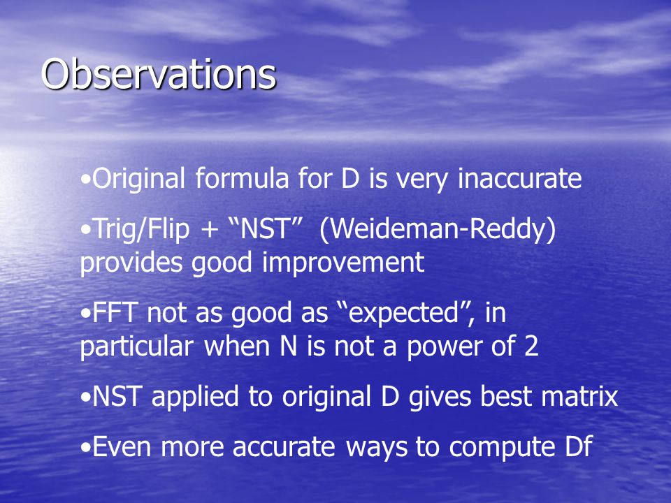
37. Observations Original formula for D is very inaccurate Trig/Flip + “NST” (Weideman-Reddy) provides good improvement FFT not as good as “expected”, in particular when N is not a power of 2 NST applied to original D gives best matrix Even more accurate ways to compute Df

38. Machine Dependency Results can vary substantially from machine to machine, and may depend on software. Intel/PC: FFT performs better SGI SUN DEC Alpha

39. Understanding the Negative sum trick

40. Error in D Error in f

41. Understanding NST 2

42. Understanding NST 3 The inaccurate matrix elements are multiplied by very small numbers leading to O(N 2 ) errors -- optimal accuracy

43. Understanding the Negative sum trick NST is an (inaccurate) implementation of the Schneider-Werner formula: Schneider-Werner Negative Sum Trick

44. Understanding the Negative sum trick Why do we obtain superior results when applying the NST to the original (inaccurate) formula? Accuracy of Finite Difference Quotients:

45. Finite Difference Quotients For monomials a cancellation of the cancellation errors takes place, e.g.: Typically f j – f k is less accurate than x j – x k, so computing x j - x k more accurately does not help!

46. Finite Difference Quotients

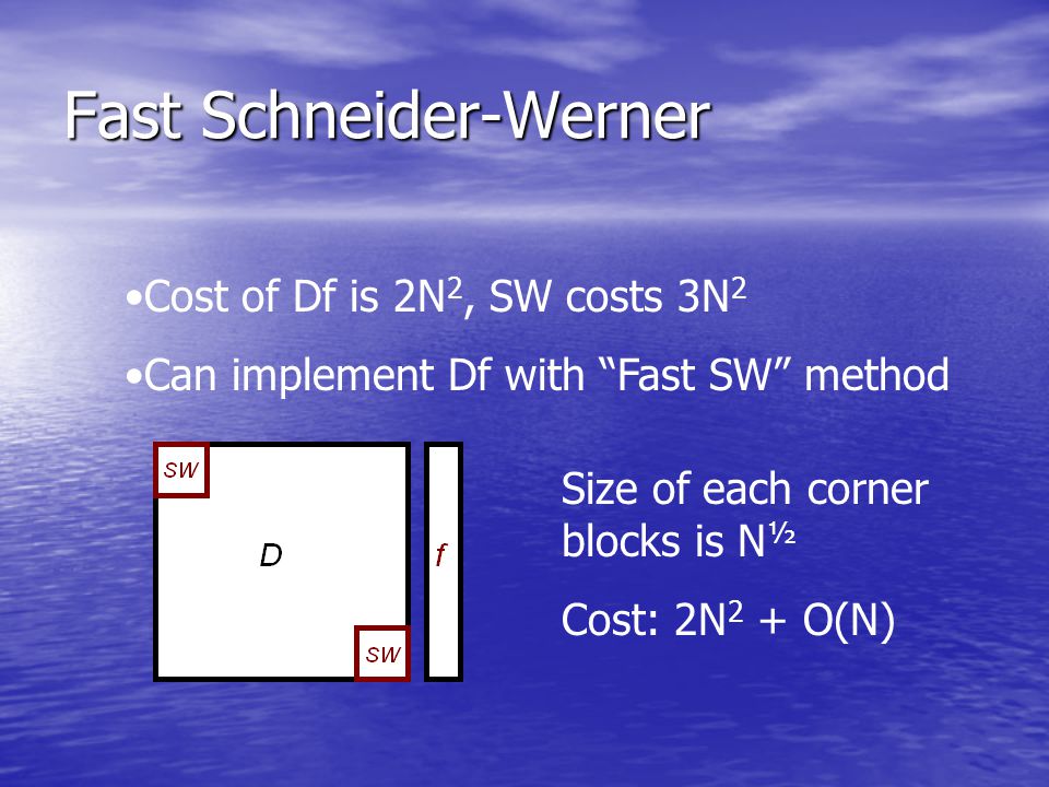
48. Fast Schneider-Werner Cost of Df is 2N 2, SW costs 3N 2 Can implement Df with “Fast SW” method Size of each corner blocks is N ½ Cost: 2N 2 + O(N)

49. Polynomial Differentiation For example, Legendre, Hermite, Laguerre For example, Legendre, Hermite, Laguerre Fewer tricks available, but Negative Sum Trick still provides improvements Fewer tricks available, but Negative Sum Trick still provides improvements Ordering the summation may become even more important Ordering the summation may become even more important

50. Higher Order Derivatives Best not to compute D (2) =D 2, etc. Best not to compute D (2) =D 2, etc. Formulas by Welfert (implemented in Weideman-Reddy) Formulas by Welfert (implemented in Weideman-Reddy) Negative sum trick shows again improvements Negative sum trick shows again improvements Higher order differentiation matrices badly conditioned, so gaining a little more accuracy is more important than for first order Higher order differentiation matrices badly conditioned, so gaining a little more accuracy is more important than for first order

51. Using D to solve problems In many applications the first and last row/column of D is removed because of boundary conditions In many applications the first and last row/column of D is removed because of boundary conditions f -> Df appears to be most sensitive to how D is computed (forward problem = differentiation) f -> Df appears to be most sensitive to how D is computed (forward problem = differentiation) Have observed improvements in solving BVPs Have observed improvements in solving BVPs Skip

52. Solving a Singular BVP

53. Results Results

54. Close Demystified some of the less intuitive behaviour of differentiation matrices Demystified some of the less intuitive behaviour of differentiation matrices Get more accuracy for the same cost Get more accuracy for the same cost Study the effects of using the various differentiation matrices in applications Study the effects of using the various differentiation matrices in applications Forward problem is more sensitive than inverse problem Forward problem is more sensitive than inverse problem Df: Time-stepping, Iterative methods Df: Time-stepping, Iterative methods

55. To think about Is double precision enough as we are able to solve “bigger” problems? Is double precision enough as we are able to solve “bigger” problems? Irony of spectral methods: Exponential convergence, round-off error is the limiting factor Irony of spectral methods: Exponential convergence, round-off error is the limiting factor Accuracy requirements limit us to N of moderate size -- FFT is not so much faster than matrix based approach Accuracy requirements limit us to N of moderate size -- FFT is not so much faster than matrix based approach

56. And now for the twist….