1. 1 The Nature of Particulate Pollutants 朱信 Hsin Chu Professor Dept. of Environmental Engineering National Cheng Kung University

2. 2 1. Primary and Secondary Particles Next slide (Fig. 8.1) An overview of particles and their properties.Fig. 8.1 “ diameter ” for a nospherical particle means “ diameter of a sphere of equal volume ”.volume

4. 4 The particles that cause significant air pollution problems are generally in the size range 0.01 to 10 µ. Particles diameters are also stated in terms of Tyler screen size in the United States, e.g., the sieve size of Tyler 100 mesh screen is equivalent to 150 µ.

5. 5 Some industrial particulate pollutants (e.g., pulverized coal, which has a size range of 3 to 400 µ ) may be created mechanically but most crushing and grinding processes do not produce particles smaller than about 10 µ. Instead, most of the fine particles (0.1 to 10 µ ) shown on the figure are obtained by combustion, evaporation, or condensation processes.

6. 6 One example is the formation of tobacco smoke, which is shown in Fig. 8.1 as having a size range from 0.01 to 1 µ. Next slide (Fig. 8.2) The cigarette smoke consists of droplets of condensed hydrocarbons (oils, tars).Fig. 8.2oils, tars

8. 8 The finest particles that have been made for research purposes are made by heating a metal or a salt to it vaporization temperature and then condensing the resulting gaseous metal or salt by quickly cooling it so that many small particles (0.01 µ ) form rather than a few large ones.

9. 9 It is uncommon in the air pollution literature to distinguish between fine particles that are solids and liquids (e.g., tars). In the atmosphere and in common collecting devices they frequently behave alike.

10. 10 Most fuels contain some incombustible materials, which remain behind when the fuel is burned, called ash. The ash left behind by the combustion of wood, coal, or charcoal contains mostly the oxides of silicon, calcium, and aluminum, with traces of other minerals.

11. 11 The distinction between mechanical and condensed particles is illustrated by tests in which pulverized lignite was burned in a laboratory furnace. The ash particles in the exhaust gases consisted of two groups. One group had an average diameter of about 0.02 µ, the other about 10 µ.

12. 12 The smaller particles contained a much higher percentage of the more volatile materials in the ash (P, Mg, Na, K, Cl, Zn, Cr, As, Co, and Sb) than did the larger particles. Almost certainly the fine particles were formed by condensation, in the furnace, of materials that had been vaporized during the combustion process.

13. 13 The larger particles were formed from the remaining mineral matter in the fuel that was not vaporized. Next slide (Fig. 8.3) A sample of particles collected from a coal-fired furnace operated at fuel-rich conditions, resulting in significant unburned carbon in the fly ash.Fig. 8.3fly ash

15. 15 The spherical particles in Fig. 8.3a are parts of the coal ’ s mineral ash which melted in the furnace and were drawn into spherical shapes by surface tension. The irregular, porous particles (like the large one at the lower left of Fig. 8.3a) are pieces of coal char, which in mostly carbon plus the mineral ash.

16. 16 The large piece at the top of Fig, 8.3a is soot, which forms long, lacy filaments up to a few millimeters long. At high magnification (Fig. 8.3b) one can see that the soot is an agglomerate of spherical particles, typically 0.01 to 0.03 microns in diameter.

17. 17 If enough excess air had been supplied and enough time allowed, we would expect that all the char and soot would have burned, and only the spherical metal oxide ash particles would have remained. Fig. 8.4 (next slide) shows an example of that type of ash. The largest particle is roughly 20 µ in diameter, the smallest visible particles are about 0.3 µ in diameter.next slidediameter

19. 19 Another property of fine particles that is different from our experience with particles as large as sand grains is that when two fine particles are brought into direct physical contact, they generally will stick together by electrostatic and van der Waals bonding forces.

20. 20 Electrostatic and van der Waals forces are, in general, proportional to the surface area of the particle. Gravity and inertial forces are proportional to the particle mass, which is proportional to D 3, whereas the surface area are proportional to D 2.

21. 21 Thus, as the particle size decreases, D 3 goes down much faster than D 2 so that the ratio of electrostatic and van der Waals to inertial and gravity forces becomes larger. As a result, if you had a handful of 1- µ particles that had been brought together into intimate contact and threw them into the air, they would not fragment into individual 1 µ particles but rather would break up into agglomerates that are the size of ordinary sand (several hundred µ ).

22. 22 For this reason, the basic strategy of control for particulate pollutants is to agglomerate them into larger particles that can be easily collected. This can be done by forcing the individual particles to contact each other (as in settling chambers, cyclones, electrostatic precipitators, or filters) or by contacting them with drops of water (as in wet scrubbers).

23. 23 The particulate pollutants can be formed in the atmosphere from gaseous pollutants, e.g., hydrocarbons, oxides of nitrogen, and oxides of sulfur. These particles are often called secondary particles, to distinguish them from those found in the atmosphere in the form in which they were emitted, which are called primary particles.

24. 24 From Fig. 8.1, we see the wavelengths of visible light are about 0.4 to 0.8 µ. Particles in this size range are the most efficient light-scatterers. The hazy days and visible smog that occur in our cities are largely caused by secondary particles that tend to form in this size range.

25. 25 Near the middle of Fig. 8.1 we see “ Lung- damaging dust ”, which has sizes from about 0.5 to 5 µ. Tests show that particles larger than about 10 µ are removed in our noses and throats; very few get into the trachea or bronchi.

26. 26 Particles in the size range 5 to 10 µ are mostly removed in the trachea and bronchi and do not get to the lungs. Some researchers use the term inhalable particles to refer to all particles smaller than 10 µ m and respirable particles to refer to those smaller than 3.5 µ.

27. 27 2. Settling Velocity and Drag Forces The second row from the bottom of Fig. 8.1 shows the “ terminal gravitational settling velocity ” for spheres of specific gravity 2.0. We can see that the value for a coarse sand grain with a diameter of 1,000 µ in air is 6 m/s. This is much higher than the common vertical wind velocities of the atmosphere, so that it is rare for the wind to blow such particles up or to hold them up once they are in the air.

28. 28 The terminal settling velocity of a 1- µ diameter particle is 6 × 10 -5 m/s. The vertical movements of outdoor air (and even the air in most rooms) normally exceed this value, so particles this size do not quickly settle out of the atmosphere.

29. 29 Thus, we distinguish between dust, which settles out of the atmosphere quickly because of its high gravitational settling velocity, and suspendable particles, which settle so slowly that they may be considered to remain in the atmosphere until they are removed by precipitation.

30. 30 There is no clear and simple dividing line between the two categories, but if we must make such an arbitrary distinction, it would be made somewhere near a particle diameter of 10 µ. Particles small enough to remain suspended in the atmosphere or in other gases for long times are called aerosols, which indicates that they behave as if they were dissolved in the gas.

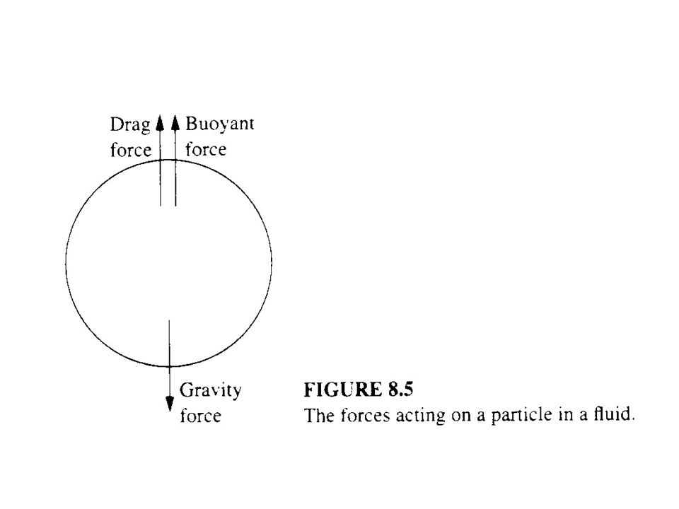
31. 31 2.1 Stokes ’ Law Next slide (Fig. 8.5) The forces acting on a spherical particle settling through a fluid under the influence of gravity.

33. 33 Writing Newton ’ s law for the particle, we obtain (1) The three terms on the right represent, respectively, the gravity, buoyant, and drag forces acting on the particle.

34. 34 The drag (or air resistance) forces increase with increasing speed and are zero for zero speed. The particle accelerates rapidly; as it accelerates, the drag force increases as the velocity increases, until it equals the gravity force minus the buoyant force. At this terminal settling velocity, the sum of the forces acting is zero, so the particle continues to move at a constant velocity.

35. 35 To find this velocity, we set the acceleration to zero in Eq. (1) and find (2) To find the velocity, we need the relation between F d and the velocity.

36. 36 Stokes worked this out mathematically for a set of assumptions that are generally quite good for most of the problems in this course, finding where µ = the viscosity of the fluid. If we substitute Eq. (3) into Eq. (2) and solve for v, we find which is commonly referred to Stokes ’ law.

37. 37 Example 1 Compute the terminal settling velocity in air of a sphere with diameter 1 µ. Solution: Finding the properties of air and of particles, then, substituting those values in Eq. (4), we find

38. 38 Stokes ’ law has been well verified for the range of conditions in which its assumptions hold good. However, for both very large and very small particles these assumptions break down. The situation is illustrated in Fig. 8.6 (next slide).

40. 40 2.2 Particles Too Large for Stokes ’ Law At larger particle sizes, the flow of fluid around the sphere becomes turbulent and the principal assumptions of Stokes ’ law then become inapplicable. Although various efforts have been made to derive a formula equivalent to Eq. (3) for larger particles, no theoretical formula represents experimental data over more than a modest range of values.

41. 41 However, the experimental data can be easily correlated by a nondimensional relationship. A new parameter, called the drag coefficient C d, is defined by Eq. (5): (5)

42. 42 In addition, we introduce the Reynolds number for a particle: (6) The Reynolds number is a dimensionless ratio of the inertial forces acting on a mass of fluid to the viscous forces acting on the same mass of fluid in the same flow.

43. 43 There are theoretical grounds for smooth spheres in uniform, subsonic flow in constant- density Newtonian fluids, the drag coefficient should depend on the Reynolds number alone. Thus, on a plot of C d versus R p, all the data for all sizes of spheres and all constant-density Newtonian fluids should fall on a single curve.

44. 44 The reader may verify that the Stokes ’ drag term (Eq.(3)) can be substituted in Eq. (5) and the result rewritten as C d = 24/R p. Experimentally, it has been found that Stokes ’ law represents the observed behavior of particles satisfactorily for Reynolds numbers less than about 0.3.

45. 45 For the 0.3 ≤ R P ≤ 1,000, the experimental drag coefficient data can be represented with satisfactory accuracy by the following empirical, data-fitting equation: (7)

46. 46 Example 2 A spherical particle with diameter 200 µ is falling in air. If Stokes were correct for this particle, how fast would it be falling, and what would its Reynolds number be? Solution: We can take our result from Example 1, if Stokes ’ law applies, then the velocity is proportional to the diameter squared, so

47. 47 This result is clearly greater than the Reynolds number of 0.3, which is the normal upper limit for reliable use of Stokes ’ law.

48. 48 Example 3 Estimate the true settling velocity of the 200- µ diameter particle in Example 2 using the experimental drag coefficient correlation in Eq. (7). Solution: In this case we must use a trial-and-error solution because we do not know the real Reynolds number.

49. 49 We begin by assuming that the particle Reynolds number is 20. then from Eq. (7) we see that Solving Eq. (5) for the velocity:

50. 50 Here, at the terminal settling velocity, F d = mg = (π/6)D 3 ρ p g. Thus, Now we must check our assumption that R p = 20.

51. 51 From Eq. (7) we compute that this corresponds to C d =2.82. Since the calculated v t is proportional to (1/C d ) 1/2, we can compute the new estimate of the terminal velocity as Repeating the R p calculation, we find R p =16.5.

52. 52 For this R p, Eq. (7) shows a C d of about 2.90 leading to a new velocity estimate of 1.22 m/s and a new R p of 16.2. At this point, we may consider the problem solved. #

53. 53 Example 3 shows the following: (1)For a 200- µ particle of specific gravity 2 settling in air at 20 o C, the true velocity is only 50% (=1.22/2.42) of the velocity calculated by Stokes ’ law. (2)This type of calculation by trial and error is tedious.

54. 54 Next slide (Fig. 8.7) A plot similar to Fig. 8.6, but it covers a range of particle density and also shows particle settling velocity in water.

56. 56 2.3 Particles Too Small for Stokes ’ Law Stokes ’ law assumes that the fluid in which the particle is moving in a continuous medium. When a particle becomes as small as or smaller than the average distance between molecules, then its interaction with molecules changes.

57. 57 At this circumstance, the number of collisions of molecules on the particle is small, some significant fraction of the colliding gas molecules are adsorbed onto the surface of the particle and remain long enough to “ forget ” what direction they came from. In this case their direction of leaving is diffuse, meaning random, subject to some statistical rules.

58. 58 The effect of the change from specular to diffuse reflection is to lower the drag force, which causes the particle to move faster. The most widely used correction factor for this change has the form (8) whereA=an experimentally determined constant λ=mean free path (the average travel distance of a gas molecule between successive collisions) F d-Stoke =the drag force computed according to Stokes ’ law

59. 59 The (1+Aλ/D) term used here is commonly called Cunningham correction factor. It is only applicable for values of λ/D of order of magnitude one. For much larger value of λ/D, more complex formulae are used.

60. 60 Most workers use the value of A in Eq. (8) found by Millikan for oil droplets settling in air, A=1.728. This is not derived theoretically, nor is it necessarily applicable to other kinds of particles or other gases but it is widely used because we do not have better information.

61. 61 Example 4 A spherical particle with diameter 0.1 µ is settling in still air. What is its terminal settling velocity? Solution: By combining Eqs (3) and (8), we find v = v Stokes (1 + Aλ/D) We find that v Stokes is our answer from Example 1, divided by 100, v Stokes = 6.5 x 10 -7 m/s

62. 62 The mean free path λ depends on T, P, and M. For air at one atmosphere and room temperature λ ≈ 0.07 µ, so and

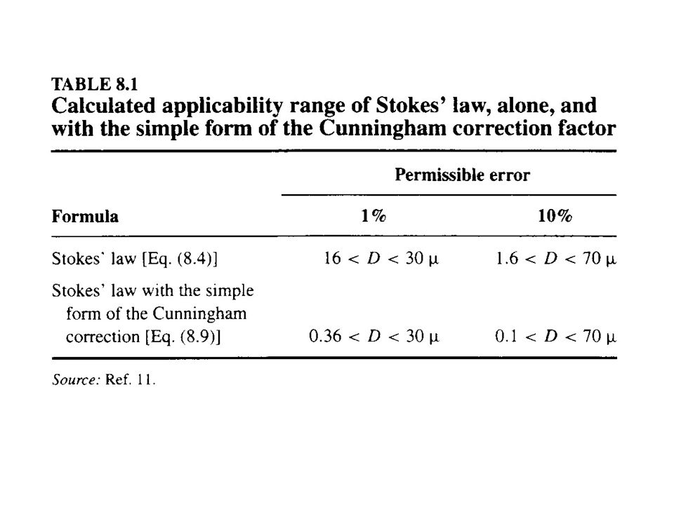
63. 63 For oil droplets Fuchs suggested the limits listed in Table 8.1 (next slide) for errors in the applicability of Stokes ’ law, and Stokes ’ law modified by the simple form of the Cunningham correction factor.next slide correction factor

65. 65 Since most of the industrial particle collectors work on particles with diameters in the range of 1.6 to 70 µ, most are designed on the basis of Stokes ’ law in the early stages. For the final design calculation, the Cunningham correction factor is used as well.

66. 66 2.4 Stokes Stopping Distance Example 5 A 1 µ diameter spherical particle with specific gravity 2.0 is ejected from a gun into standard air at a velocity of 10 m/s. How far does it travel before it is stopped by viscous friction? Here we ignore the effect of gravity.

67. 67 Solution: The drag force is the only force acting on the particle after it leaves the gun. Where C is the Cunningham correction factor. Thus,

68. 68 Substituting dt = dx/v, separating variables, canceling the two v terms, and intergrating, we find and

69. 69 2.5 Aerodynamic Particle Diameter Eq. (9) also shows that any two particles that have the same value of D 2 ρ p C will have the same Stokes stopping distance for any initial velocity (in air with the same viscosity). They have the same aerodynamic behavior.

70. 70 For that reason, we define a new property, the aerodynamic particle diameter: D a =D(ρ p C) 1/2 This is a peculiar diameter, because it has the dimensions [(length)(mass/length 3 ) 1/2 ], e.g., [(m)(kg/m 3 ) 1/2 ].

71. 71 Thus the particle in Example 5 would have an aerodynamic particle diameter, D a, of Where the symbol µ a stands for “ microns, aerodynamic ”. In SI units this should be stated as 0.21 µ m (1000 kg/m 3 ) 0.5, but that usage is seldom seen.

72. 72 2.6 Diffusion of Particles Small particles move by Brownian motion, which we describe according to the equations for diffusion. If the particle is small enough that it can only expect a few collisions with the surrounding gas molecules per second and its inertia is small because of its small size, then the force of an individual collision is enough to make it move.

73. 73 Subsequent collisions, whose directions are random, will move it in other directions, so that its time-series path will be a series of short jumps in one direction and then another. In a uniform solution or suspension, Brownian motion does not cause any net change in the concentration with time in any part of the solution.

74. 74 But if the concentration is not uniform, then Brownian motion tends to equalize the concentration. From diffusion theory, we know that for three- dimensional, nonsteady-state diffusion (10) WhereD =diffusivity (normal units m 2 /s) c =concentration

75. 75 For steady-state, one-dimensional diffusion Eq. (10) reduces to the well-known Fick ’ s law of diffusion For spherical particles suspended in a perfect gas, D may be estimated from the kinetic theory of gases as wherek =Boltzmann constant C =Cunningham correction factor

76. 76 Example 6 Estimate the diffusivity of a 1- µ diameter particle in air at 20 o C and 1 atm. Solution: For a 1- µ diameter particle the Cunningham correction factor can be shown from Eq. (8) to be about 1.16, so

77. 77 Most gases diffuse in air with diffusivities of about 10 -5 m 2 /s, and diffusivities of solutes in liquids are typically about 10 -9 m 2 /s. Thus, particles on the order of a few microns do not diffuse rapidly.