Download presentation
Presentation is loading. Please wait.

1
Viscoelastic Characterization
Dr. Muanmai Apintanapong

2
Elastic deformation - Flow behavior

3
Elastic behavior

4
Newtonian behavior

5
Newtonian liquid

7
.

8
Introduction to Viscoelasticity
All viscous liquids deform continuously under the influence of an applied stress – They exhibit viscous behavior. Solids deform under an applied stress, but soon reach a position of equilibrium, in which further deformation ceases. If the stress is removed they recover their original shape – They exhibit elastic behavior. Viscoelastic fluids can exhibit both viscosity and elasticity, depending on the conditions. Viscous fluid Viscoelastic fluid Elastic solid

9
Shear Stress

10
Shear Rate

11
Practical shear rate values

12
Viscosity =resistance to flow

13
Viscosity of fluids at 20C
Go to stress relaxation

14
Viscosity: temperature dependence

15
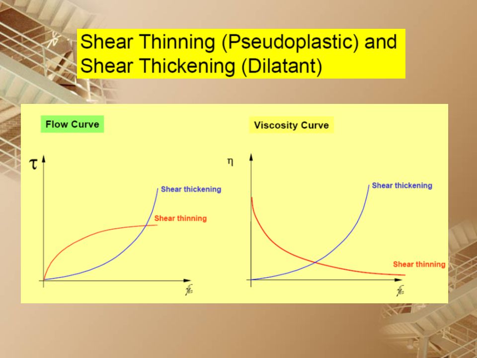
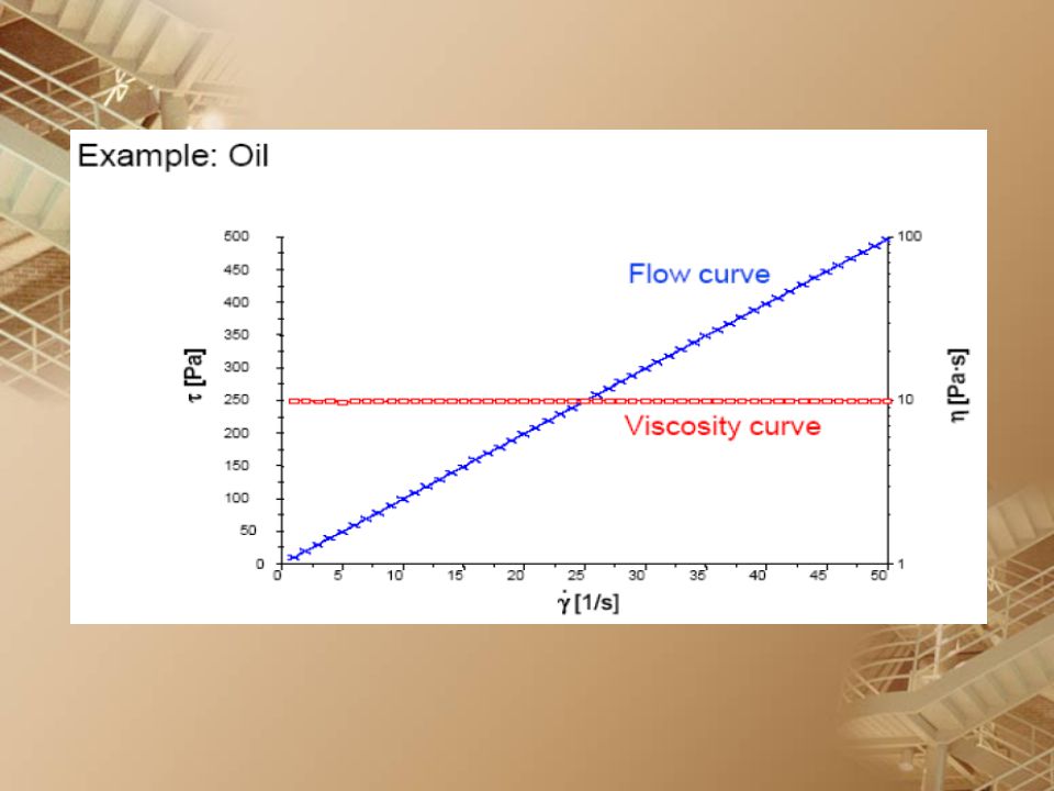
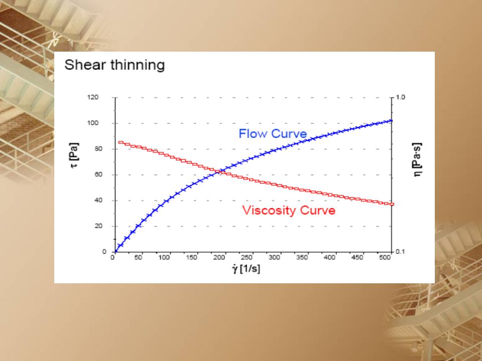
Flow curve and Viscosity curve

17
Flow behavior: flow curve

18
Flow behavior: viscosity curve

25
Universal Testing Machine
Stress Relaxation Force sensor Instron, TA XT2 Universal Testing Machine

26
Stress Relaxation Test
Strain Elastic Stress Stress Viscoelastic Stress Viscous fluid Viscous fluid Viscous fluid Time, t

27
Stress Relaxation Experiment
Strain is applied to sample instantaneously (in principle) and held constant with time. Stress is monitored as a function of time (t). Strain time
 and held constant with time. Stress is monitored as a function of time (t). Strain. time.")
28
Stress Relaxation Experiment
Response of Classical Extremes Elastic Viscous Hookean Solid Newtonian Fluid Stress Stress stress for t>0 is 0 stress for t>0 is constant time time Stress decreases with time starting at some high value and decreasing to zero. Response of Material Visco elastic Stress time

29
Creep Recovery Experiment
Stress is applied to sample instantaneously, t1, and held constant for a specific period of time. The strain is monitored as a function of time ((t) or (t)). The stress is reduced to zero, t2, and the strain is monitored as a function of timetort Stress t1 t2 time
 or (t)). The stress is reduced to zero, t2, and the strain is monitored as a function of timetort Stress. t1. t2. time.")
30
Creep Recovery Experiment
Deformation Stress t1 time t2 Response of Classical Extremes Elastic Viscous Stain rate for t>t1 is constant Strain for t>t1 increase with time Strain rate for t >t2 is 0 Stain for t>t1 is constant Strain for t >t2 is 0 Strain Strain t1 time t2 t1 time t2

31
Creep Recovery Experiment: Response of Viscoelastic Material
time t 1 2 Recoverable Strain Recovery = 0 (after steady state) / Strain rate decreases with time in the creep zone, until finally reaching a steady state. In the recovery zone, the viscoelastic fluid recoils, eventually reaching a equilibrium at some small total strain relative to the strain at unloading. Reference: Mark, J., et.al., Physical Properties of Polymers ,American Chemical Society, 1984, p. 102.
 / Strain rate decreases with time in the creep zone, until finally reaching a steady state. In the recovery zone, the viscoelastic fluid recoils, eventually reaching a equilibrium at some small total strain relative to the strain at unloading. Reference: Mark, J., et.al., Physical Properties of Polymers. ,American Chemical Society, 1984, p")
32
Creep Recovery Experiment
Recovery = 0 (after steady state) / Strain Less Elastic More Elastic Creep Zone Recovery Zone t1 t2 time
 / Strain. Less Elastic. More Elastic. Creep Zone. Recovery Zone. t1. t2. time.")
33
Rheological Models Mechanical components or elements

34
Elastic (Solid-like) Response
A material is perfectly elastic, if the equilibrium shape is attained instantaneously when a stress is applied. Upon imposing a step input in strain, the stresses do not relax. The simplest elastic solid model is the Hookean model, which we can represent by the “spring” mechanical analog.

35
Elasticity deals with mechanical properties of elastic solids (Hooke’s Law)
Stress, L Strain, = L/L L E=/

36
Stress, Strain,

37
Elastic (Solid-like) Response
Stress Relaxation experiment (stress) o (strain) to=0 to=0 time time Creep Experiment (stress) (strain) o/E o to=0 ts to=0 ts time time
 o. (strain) to=0. to=0. time. time. Creep Experiment. (stress) (strain) o/E. o. to=0. ts. to=0. ts. time. time.")
38
Viscous (Liquid-like) Response
A material is purely viscous (or inelastic) if following any flow or deformation history, the stresses in the material become instantaneously zero, as soon as the flow is stopped; or the deformation rate becomes instantaneously zero when the stresses are set equal to zero. Upon imposing a step input in strain, the stresses relax as soon as the strain is constant. The liquid behavior can be simply represented by the Newtonian model. We can represent the Newtonian behavior by using a “dashpot” mechanical analog:
 if following any flow or deformation history, the stresses in the material become instantaneously zero, as soon as the flow is stopped; or the deformation rate becomes instantaneously zero when the stresses are set equal to zero. Upon imposing a step input in strain, the stresses relax as soon as the strain is constant. The liquid behavior can be simply represented by the Newtonian model. We can represent the Newtonian behavior by using a dashpot mechanical analog:")
39
Theory of Hydrodynamics
Newton’s Law In Newtonian Fluids, Stress is proportional to rate of strain but independent of strain itself

40
Stress, Strain, ,

41
Viscous (Liquid-like) Response
Stress Relaxation experiment (suddenly applying a strain to the sample and following the stress as a function of time as the strain is held constant). o (strain) (stress) to=0 to=0 time time Creep Experiment (a constant stress is instantaneously applied to the material and the resulting strain is followed as a function of time) t (stress) (strain) to ts ts to=0 time to=0 time
. o. (strain) (stress) to=0. to=0. time. time. Creep Experiment (a constant stress is instantaneously applied to the material and the resulting strain is followed as a function of time) t (stress) (strain) to. ts. ts. to=0. time. to=0. time.")
42
Energy Storage/Dissipation
Elastic materials store energy (capacitance) Viscous materials dissipate energy (resistance) Energy t Energy t E Viscoelastic materials store and dissipate a part of the energy t
 Viscous materials dissipate energy (resistance) Energy. t. Energy. t. E. Viscoelastic materials store and. dissipate a part of the energy. t.")
43
What causes viscoelastic behavior?
Energy Storage +Dissipation Food Chemists – More on nature of these polymers Reference: Dynamics of Polymeric Liquids (1977). Bird, Armstrong and Hassager. John Wiley and Sons. pp: 63. Long polymer chains at the molecular scale, make polymeric matrix viscoelastic at the microscale
. Bird, Armstrong and Hassager. John Wiley and Sons. pp: 63. Long polymer chains at the molecular scale, make polymeric matrix viscoelastic at the microscale.")
44
Specifically, viscoelasticity is a molecular rearrangement
Specifically, viscoelasticity is a molecular rearrangement. When a stress is applied to a viscoelastic material such as a polymer, parts of the long polymer chain change position. This movement or rearrangement is called Creep. Polymers remain a solid material even when these parts of their chains are rearranging in order to accompany the stress, and as this occurs, it creates a back stress in the material. When the back stress is the same magnitude as the applied stress, the material no longer creeps. When the original stress is taken away, the accumulated back stresses will cause the polymer to return to its original form. The material creeps, which gives the prefix visco-, and the material fully recovers, which gives the suffix –elasticity.

45
Examples of viscoelastic foods:
Almost all solid foods and fluid foods containing long chain biopolymers Food starch, gums, gels Grains Most solid foods (fruits, vegetables, tubers) Cheese Pasta, cookies, breakfast cereals
 Cheese. Pasta, cookies, breakfast cereals.")
46
Viscoelasticity Experiments
Static Tests Stress Relaxation test Creep test Dynamic Tests Controlled strain Controlled stress (When we apply a small oscillatory strain and measure the resulting stress)
")
47
Why we want to fit models to viscoelastic test data?
To quantify the data – mathematical representation For use with other food processing applications Some food drying models require viscoelastic properties Design of pipelines, mixing vessels etc., using viscoelastic fluid foods To obtain information at different test conditions Example: Extrusion To obtain an estimate of elastic properties and relaxation times Helps to quantify glass transition

48
Viscoelastic Models Maxwell Model Kelvin-Voigt Model
Used for stress relaxation tests Used for creep tests

49
Viscoelastic Response – Maxwell Element
A viscoelastic material (liquid or solid) will not respond instantaneously when stresses are applied, or the stresses will not respond instantaneously to any imposed deformation. Upon imposing a step input in strain the viscoelastic liquid or solid will show stress relaxation over a significant time. At least two components are needed, one to characterize elastic and the other viscous behavior. One such model is the Maxwell model:
 will not respond instantaneously when stresses are applied, or the stresses will not respond instantaneously to any imposed deformation. Upon imposing a step input in strain the viscoelastic liquid or solid will show stress relaxation over a significant time. At least two components are needed, one to characterize elastic and the other viscous behavior. One such model is the Maxwell model:")
50
Viscoelastic Response
Strain, Stress, Let’s try to deform the Maxwell element

51
Maxwell Model Response
The Maxwell model can describe successfully the phenomena of elastic strain, creep recovery, permanent set and stress relaxation observed with real materials Moreover the model exhibits relaxation of stresses after a step strain deformation and continuous deformation as long as the stress is maintained. These are characteristics of liquid-like behaviour Therefore the Maxwell element represents a VISCOELASTIC FLUID.

52
Maxwell Model-when is applied
1. will be same in each element 2. Total = sum of individual

53
Maxwell Model Response
1) Creep Experiment: If a sudden stress is imposed (step loading), an instantaneous stretching of the spring will occur, followed by an extension of the dashpot. Deformation after removal of the stress is known as creep recovery: . Or by defining the “creep compliance”: Elastic Recovery (stress) o/E Permanent Set dashpot o o/E spring to=0 ts to=0 ts time time
 Creep Experiment: If a sudden stress is imposed (step loading), an instantaneous stretching of the spring will occur, followed by an extension of the dashpot. Deformation after removal of the stress is known as creep recovery: . Or by defining the creep compliance : Elastic Recovery. (stress) o/E. Permanent. Set. dashpot. o. o/E. spring. to=0. ts. to=0. ts. time. time.")
54
Maxwell Model Response
2) Stress Relaxation Experiment: If the mechanical model is suddenly extended to a position and held there (o=const., =0): . Exponential decay Also recall the definition of the “relaxation” modulus: and (stress) time to=0 o=Goo o (strain) to=0 time = /E = Relaxation time = the time required by biopolymers to relax the stresses
 Stress Relaxation Experiment: If the mechanical model is suddenly extended to a position and held there (o=const., =0): . Exponential decay. Also recall the definition of the relaxation modulus: and. (stress) time. to=0. o=Goo. o. (strain) to=0. time. = /E = Relaxation time = the time required by biopolymers to relax the stresses.")
55
Generalized Maxwell Model
The Maxwell model is qualitatively reasonable, but does not fit real data very well. Instead, we can use the generalized Maxwell model 1 2 3 n E1 E2 E3 En

56
Generalized Maxwell Model Applied for stress relaxation test

57
Determination of parameters for Generalized Maxwell Model
There are 4 methods. Method of Instantaneous Slope Method of Central Limit Theorem Point of Inflection Method Method of Successive Residuals direct method and more popular Optional

58
Method of Successive Residuals
First plot-semilog plot: if it is linear, use single Maxwell Model If it is not linear, use Generalized Maxwell Model

59
Plot until it is straight
time to=0 ln First plot Slope of straight line = -1/1 ln 1 Divided into many parts and plot of each part until the curvature disappears. ln Second plot Slope of straight line = 1/2 ln 2 to=0 time Plot until it is straight

60
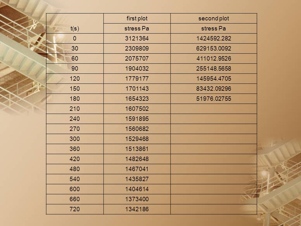
Example: Genealized maxwell model for stress relaxation test
t (min) F (kg) 100 0.5 74 1 66.5 1.5 61 2 57 2.5 54.5 3 53 3.5 51.5 4 51 4.5 50 5 49 6 48.5 7 47.5 8 47 9 46 10 45 11 44 12 43 Test sample has 2 cm diameter and 4 cm long Area = X 10-4 m2
 F (kg) Test sample has 2 cm diameter and 4 cm long. Area = X 10-4 m2.")
61
first plot ln 1= =y-intercept 1= slope= 1= second plot ln 2= =y-intercept 2= slope= 2=

62
first plot second plot t(s) stress Pa 30 60 90 120 150 180 210 240 270 300 360 420 480 540 600 660 720
63
Voigt-Kelvin Model Response
The Voigt-Kelvin element does not continue to deform as long as stress is applied, rather it reaches an equilibrium deformation. It does not exhibit any permanent set. These resemble the response of cross-linked rubbers and are characteristics of solid-like behaviour Therefore the Voigt-Kelvin element represents a VISCOELASTIC SOLID. The Voigt-Kelvin element cannot describe stress relaxation. Both Maxwell and Voigt-Kelvin elements can provide only a qualitative description of the response Various other spring/dashpot combinations have been proposed.

64
Viscoelastic Reponse Voigt-Kelvin Element
The Voigt-Kelvin element consists of a spring and a dashpot connected in parallel. E

65
Creep Recovery Experiment: applied 0 (step loading)
(strain) (strain) + to=0 to=0 time time time t Slope=/ Strain (t) 0/E = /E = characteristic time = time of retardation
 (strain) + to=0. to=0. time. time. time. t. Slope=/ Strain (t) 0/E. = /E = characteristic time = time of retardation.")
66
Generalized Voigt-Kelvin Model

67
Three element Model Standard linear solid

68
Four element Model (strain) E1 E2 2 1 spring (strain) Kevin
time to=0 o E1 E2 2 1 spring (strain) time to=0 Kevin (strain) time to=0 dashpot
 time. to=0. Kevin. (strain) time. to=0. dashpot.")
69
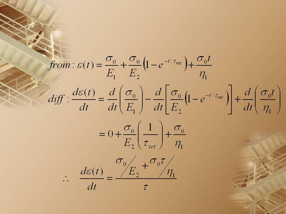
Creep test: use 4-element model
Strain (t) Slope = 0/1 . A Dashpot, 1 . . 0/E2 =r Kelvin, 2/E2 C B 0/E1= 0 Spring, E1 t time a = 2/E2=ret
 Slope = 0/1. . A. Dashpot, 0/E2 =r. Kelvin, 2/E2. C. B. 0/E1= 0. Spring, E1. t. time. a = 2/E2=ret.")
71
Generalized four-element model
Combination of four-element model in series

72
Example Analyze the given experimental creep curve in terms of the parameters of a 4-element model. Cylindrical specimen (2 cm in diameter and 5 cm long) Applied step load is 10 kg.
 Applied step load is 10 kg.")
73
slope = s0/h1=0.0266 dashpot kelvin s0/E1=e0 =0.2 spring
=er= 0.125 kelvin s0/E1=e0 =0.2 spring a = h2/E2=tret=0.9

74
Length = 0.05 m Diameter = 0.02 Area = m2 Load = 10 kg s0 = Pa slope = Deformation/time = 0.0266 cm/s per sec s0/h1= h1= Pa s s0/E2= 0.125 cm = 0.025 m/m E2 = a = 0.9 = h2/E2 h2= e0= 0/E1 = 0.2 0.04 E1 =

Similar presentations


>")

 1. Anderson's Theory of Faulting 2. Rheology (mechanical behavior of rocks) - Elastic: Hooke's.>")


 Spring 2008 Dr. Konstantinos A. Sierros.>")


