Download presentation
Presentation is loading. Please wait.

1
Jennifer Siegel

2
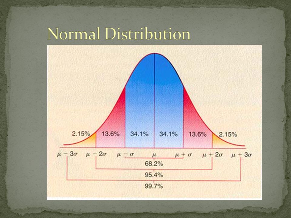
Statistical background Z-Test T-Test Anovas

3
Science tries to predict the future Genuine effect? Attempt to strengthen predictions with stats Use P-Value to indicate our level of certainty that result = genuine effect on whole population (more on this later…)
.")
5
Develop an experimental hypothesis H0 = null hypothesis H1 = alternative hypothesis Statistically significant result P Value =.05

6
Probability that observed result is true Level =.05 or 5% 95% certain our experimental effect is genuine

7
Type 1 = false positive Type 2 = false negative P = 1 – Probability of Type 1 error

9
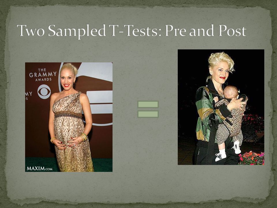
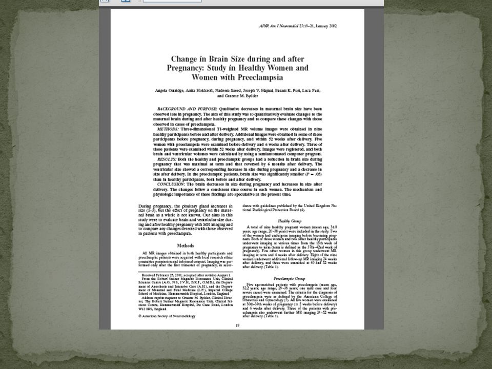
Let’s pretend you came up with the following theory… Having a baby increases brain volume (associated with possible structural changes)
")
10
Z - test T - test

11
Population

12
Cost Not able to include everyone Too time consuming Ethical right to privacy Realistically researchers can only do sample based studies

13
T = differences between sample means / standard error of sample means Degrees of freedom = sample size - 1

15
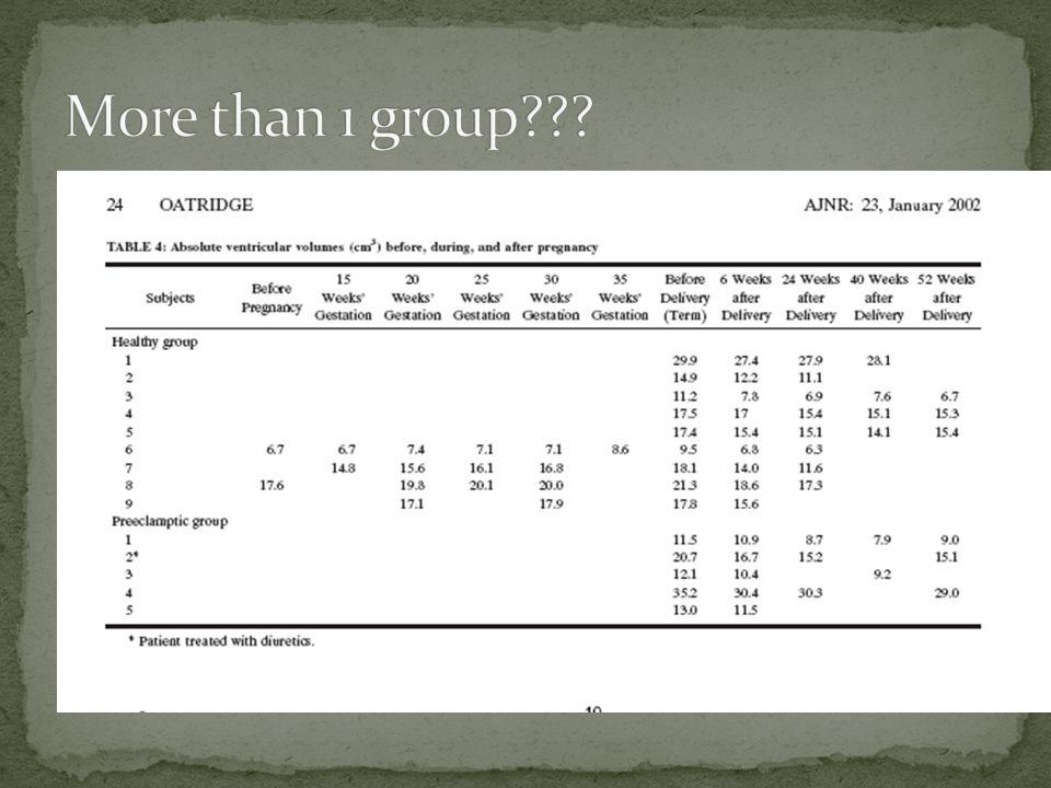
H0 = There is no difference in brain size before or after giving birth H1 = The brain is significantly smaller or significantly larger after giving birth (difference detected)
")
16
T=(1271-1236)/(119-113)
/( )")
17
http://www.danielsoper.com/statcalc/calc08.aspx Women have a significantly larger brain after giving birth

18
One-sample (sample vs. hypothesized mean) Independent groups (2 separate groups) Repeated measures (same group, different measure)
 Independent groups (2 separate groups) Repeated measures (same group, different measure).")
20
ANalysis Of VAriance Factor = what is being compared (type of pregnancy) Levels = different elements of a factor (age of mother) F-Statistic Post hoc testing
 Levels = different elements of a factor (age of mother) F-Statistic Post hoc testing")
21
1 Way Anova 1 factor with more than 2 levels Factorial Anova More than 1 factor Mixed Design Anovas Some factors are independent, others are related

22
There is a significant difference somewhere between groups NOT where the difference lies Finding exactly where the difference lies requires further statistical analysis = post hoc analysis

24
Z-Tests for populations T-Tests for samples ANOVAS compare more than 2 groups in more complicated scenarios

25
Varun V.Sethi

26
Objective Correlation Linear Regression Take Home Points.

28
Correlation - How much linear is the relationship of two variables? (descriptive) Regression - How good is a linear model to explain my data? (inferential)
 Regression - How good is a linear model to explain my data. (inferential).")
30
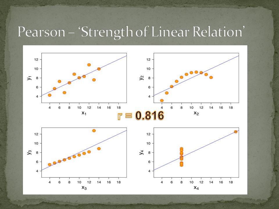
Correlation Correlation reflects the noisiness and direction of a linear relationship (top row), but not the slope of that relationship (middle), nor many aspects of nonlinear relationships (bottom).
, but not the slope of that relationship (middle), nor many aspects of nonlinear relationships (bottom).")
31
Strength and direction of the relationship between variables Scattergrams Y X YY X Y YY Positive correlationNegative correlationNo correlation

33
Measures of Correlation 1)Covariance 2) Pearson Correlation Coefficient (r)
Covariance 2) Pearson Correlation Coefficient (r)")
34
1) Covariance -The covariance is a statistic representing the degree to which 2 variables vary together {Note that S x 2 = cov(x,x) }
 Covariance -The covariance is a statistic representing the degree to which 2 variables vary together {Note that S x 2 = cov(x,x) }")
35
A statistic representing the degree to which 2 variables vary together Covariance formula cf. variance formula

36
2) Pearson correlation coefficient (r) -r is a kind of ‘normalised’ (dimensionless) covariance -r takes values fom -1 (perfect negative correlation) to 1 (perfect positive correlation). r=0 means no correlation (S = st dev of sample)
.")
38
Limitations: Sensitive to extreme values Relationship not a prediction. Not Causality

40
Regression: Prediction of one variable from knowledge of one or more other variables

41
How good is a linear model (y=ax+b) to explain the relationship of two variables? - If there is such a relationship, we can ‘predict’ the value y for a given x. (25, 7.498)
.")
42
Linear dependence between 2 variables Two variables are linearly dependent when the increase of one variable is proportional to the increase of the other one xx yy Samples: - Energy needed to boil water - Money needed to buy coffeepots

44
Fiting data to a straight line (o viceversa): Here, ŷ = ax + b – ŷ : predicted value of y – a: slope of regression line – b: intercept Residual error (ε i ): Difference between obtained and predicted values of y (i.e. y i - ŷ i ) Best fit line (values of b and a) is the one that minimises the sum of squared errors (SS error ) (y i - ŷ i ) 2 ε iε i ε i = residual = y i, observed = ŷ i, predicted ŷ = ax + b
 Best fit line (values of b and a) is the one that minimises the sum of squared errors (SS error ) (y i - ŷ i ) 2 ε iε i ε i = residual = y i, observed = ŷ i, predicted ŷ = ax + b.")
46
Adjusting the straight line to data: Minimise (y i - ŷ i ) 2, which is (y i -ax i +b) 2 Minimum SS error is at the bottom of the curve where the gradient is zero – and this can found with calculus Take partial derivatives of (y i -ax i -b) 2 respect parametres a and b and solve for 0 as simultaneous equations, giving: This can always be done
 2, which is (y i -ax i +b) 2 Minimum SS error is at the bottom of the curve where the gradient is zero – and this can found with calculus Take partial derivatives of (y i -ax i -b) 2 respect parametres a and b and solve for 0 as simultaneous equations, giving: This can always be done")
47
We can calculate the regression line for any data, but how well does it fit the data? Total variance = predicted variance + error variance s y 2 = s ŷ 2 + s er 2 Also, it can be shown that r 2 is the proportion of the variance in y that is explained by our regression model r 2 = s ŷ 2 / s y 2 Insert r 2 s y 2 into s y 2 = s ŷ 2 + s er 2 and rearrange to get: s er 2 = s y 2 (1 – r 2 ) From this we can see that the greater the correlation the smaller the error variance, so the better our prediction
 From this we can see that the greater the correlation the smaller the error variance, so the better our prediction.")
48
Do we get a significantly better prediction of y from our regression equation than by just predicting the mean? F-statistic

49
Prediction / Forecasting Quantify strength between y and Xj ( X1, X2, X3 )
")
50
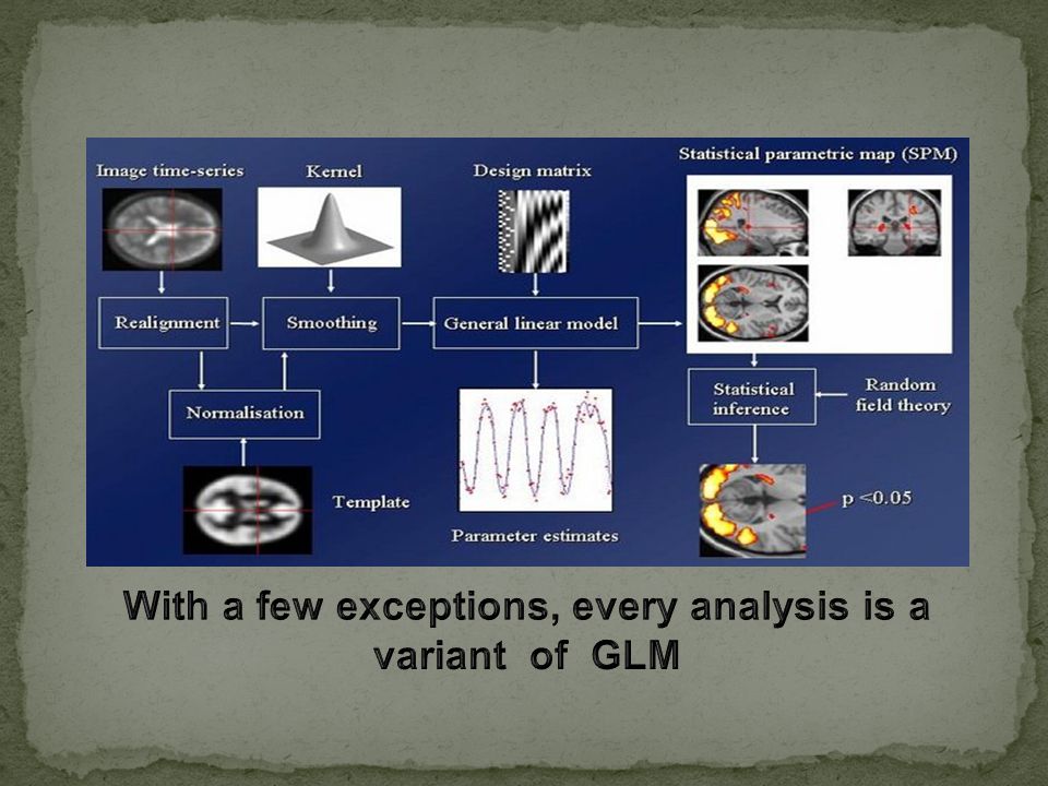
A General Linear Model is just any model that describes the data in terms of a straight line Linear regression is actually a form of the General Linear Model where the parameters are b, the slope of the line, and a, the intercept. y = bx + a +ε

51
Multiple regression is used to determine the effect of a number of independent variables, x 1, x 2, x 3 etc., on a single dependent variable, y The different x variables are combined in a linear way and each has its own regression coefficient: y = b 0 + b 1 x 1 + b 2 x 2 +…..+ b n x n + ε The a parameters reflect the independent contribution of each independent variable, x, to the value of the dependent variable, y. i.e. the amount of variance in y that is accounted for by each x variable after all the other x variables have been accounted for

52
Take Home Points - Correlated doesn’t mean related. e.g, any two variables increasing or decreasing over time would show a nice correlation: C0 2 air concentration in Antartica and lodging rental cost in London. Beware in longitudinal studies!!! - Relationship between two variables doesn’t mean causality (e.g leaves on the forest floor and hours of sun)
.")
53
Linear regression is a GLM that models the effect of one independent variable, x, on one dependent variable, y Multiple Regression models the effect of several independent variables, x 1, x 2 etc, on one dependent variable, y Both are types of General Linear Model

54
Thank You

Similar presentations


 Distributions, probabilities and P-values.>")


 measures the strength of the linear relationship.>")

![Multiple Regression [ Cross-Sectional Data ]](/15/4682560/big_thumb.jpg "Multiple Regression [ Cross-Sectional Data ]>")
 Association Between Variables Measured at the Interval-Ratio Level: Bivariate Correlation and Regression.>")


