3. What is a webcam? Webcams are small digital video cameras that hook up to your computer at the USB or Firewire port Some webcams are true CCD devices (like the Philips ToUcam) The produce 320x240 pixel images (and other resolution modes as well) They are lightweight & Cheap, $100 or so… They produce color digital video files with sound (avi file format)

4. Logitech QuickCam - one of the first to be used by amateur astronomers for Lunar and Planetary work. Philips ToUcam has been a very popular and inexpensive webcam for astronomy and is the camera I use. –an excellent entry level webcam costing around $130. There are higher performance (and much more expensive) webcams used by advanced amateurs for astronomical purposes (Luminera, DMK21F04, Point Grey). –DMK: $390 for the camera, $199 for filter wheel, $285 for filter set. –Lumenera: $995 for camera alone. –Point Grey Research has some nice fire-wire minis ~$700 or so Avoid currently available CMOS devices, they lack sensitivity compared to CCD based devices. Color vs gray-scale - filter wheels vs deBayering. Many varieties of Webcams

5. What’s Inside a typical webcam? CCD chip behind window Lens with NIR filter Video Circuit Board USB connector and cord Microphone

6. How do you use it for Astronomy? (you are going to void your warranty) Remove lens and discard Add 1.25” adapter and NIR blocking filter 1) 2) Replace eyepiece with the webcam Plug webcam into your laptop… 3) 4)

8. If you’re lucky and persistent, you will get some.avi video files of planets jiggling around with fleeting glimpses of details on the edge of visibility, a lot like what you see through the eyepiece. Wouldn’t it be great if we had some way to take the information that we know is in the video, and somehow put it all into one picture? You can also extract single frame snapshots from the video, but they tend to be blurry and don’t show the detail you glimpse in the video.

9. Here’s what Registax does: Examines every frame of your video file Does a critical evaluation of its quality. Arranges frames in order of quality Lets you pick a reference frame and how many of the best ones to keep. Aligns each frame with the reference frame Adds the frames digitally (stacking) This gives an enormous improvement in signal to noise ratio (by √n). Uses wavelet analysis to sharpen low contrast details in the image. Believe it or not. This image came from the video we saw in the previous slide! There are some details we need to deal with before we start getting pictures to rival the Hubble…. Well, thanks to a young Dutch amateur astronomer/computer programmer named Cor Berrevoets, we have a FREE downloadable program named REGISTAX which does just exactly that: http://registax.astronomy.net/html/v4_site.html

10. To get good results we need to match the resolution of the telescope to the digital sampling ability of the webcam We do this by amplfying the focal length of the telescope until the smallest resolved image details are big enough to be realistically sampled by the pixels of the webcam CCD We determine how much magnification we need using the digital sampling theorem - also the basis for high fidelity digital music recording and the operation of cell phones. Critical Details: Critically Important Factor:

11. The Digital Sampling Theorem In 1927 Harry Nyquist, an engineer at the Bell Telephone Laboratory determined the following principle of digital sampling: When sampling a signal (e.g., converting from an analog signal to digital ), the sampling frequency must be at least twice the highest frequency present in the input signal if you want to reconstruct the original perfectly from the sampled version. His work was later expanded by Claude Shannon and led to modern information theory. For this reason the theorem is now known as the Nyquist-Shannon Sampling Theorem

12. What does this all have to do with webcam astronomy? 1.The image made by the telescope optics is a two dimensional analog signal made up of spatial waveforms 2.A webcam is a digital sampling device Let’s re-state the sampling theorem in terms that relate to telescopic imaging using a webcam: The sampling frequency implied by the pixel spacing on the webcam CCD must be at least twice the highest spatial frequency present in the image to faithfully record the information in the image. If you violate this rule it’s called UNDERSAMPLING Undersampling is BAD…

13. Effects of Undersampling: 302 dpi 60 dpi 23 dpi 13 dpi Alias signals - illusions, not really there Oversampling is ok… Undersampling is not! How can we avoid undersampling in our imaging? We can illustrate this with a digital scanner and a radiating line pattern:

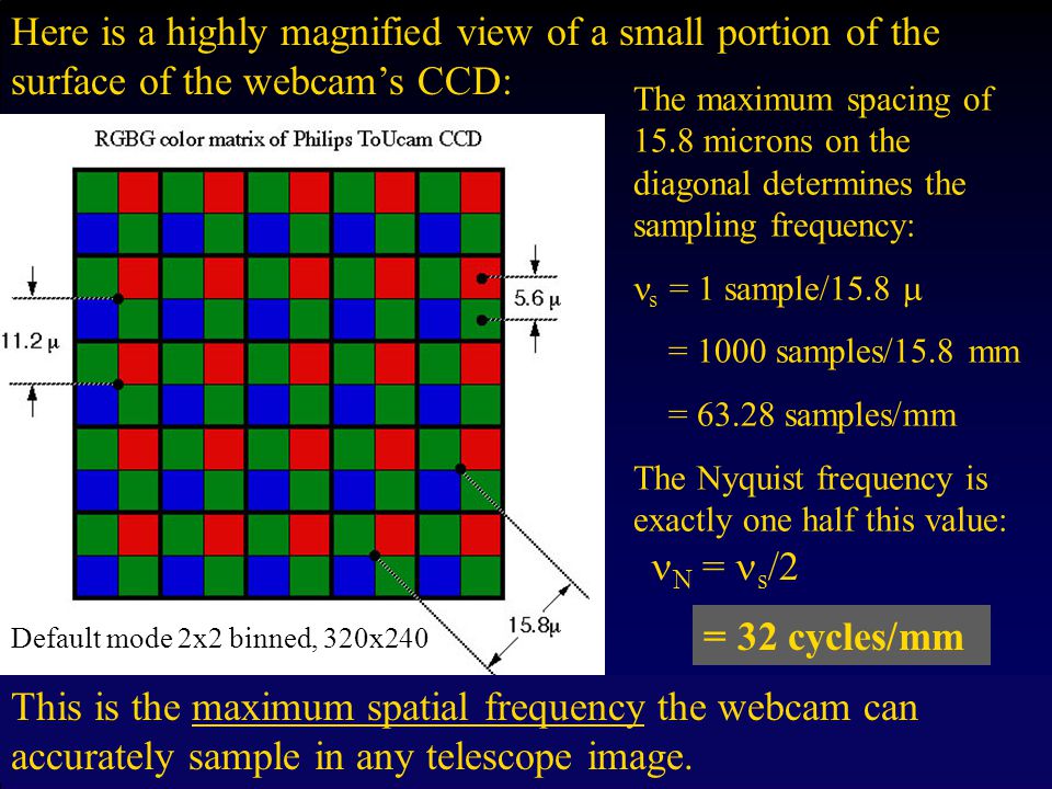
15. The maximum spacing of 15.8 microns on the diagonal determines the sampling frequency: s = 1 sample/15.8  = 1000 samples/15.8 mm = 63.28 samples/mm The Nyquist frequency is exactly one half this value: Here is a highly magnified view of a small portion of the surface of the webcam’s CCD: = 32 cycles/mm N = s /2 This is the maximum spatial frequency the webcam can accurately sample in any telescope image. Default mode 2x2 binned, 320x240

16. The maximum spacing of 11.2 microns in green pixels determines the sampling frequency for green light: s = 1 sample/11.2  = 1000 samples/11.2 mm = 89.29 samples/mm The Nyquist frequency is exactly one half this value: Here’s how the pixels are utilized in the “higher” 640x480 resolution mode: = 45 cycles/mm N = s /2 However, blue and red still have a Nyquist frequency of 32 cycles/mm 640x480 mode No binning

17. Pixels are “binned” into 4x4 pixel arrays with vertical and horizontal spacings of 22.4 microns and a diagonal spacing of 31.6 microns. The minimum sampling frequency is: s = 1 sample/31.6  = 31.64 samples/mm The Nyquist frequency is: Here’s how the pixels are utilized in the 160x120 mode: = 16 cycles/mm N = s /2 4x4 binned 160x120 pixels

18. Now let’s talk about the resolution of the telescope. First, some optical definitions: Focal length = F Aperture = D = diameter of lens or mirror Focal ratio = F/D (usually written f/# as in f/8 or f/2.5 or referred to as f-number or f-stop) image F D

19.  The diameter of the disk, , is dependant only upon the focal ratio (f # ) of the optical system and the wavelength,, of the light used:  = 2.44 f # = 1.34f # = 1.34*f# (for green light =0.55  ) Diffraction causes the image of a point source to be spread out into a circular spot called the Airy disk: Spatial Frequencies in the Telescope Image 

20. Raleigh Limit for Resolution Two points of light separated by the radius of their Airy disks can just be perceived as two points.  How do we convert this information into a spatial frequency?  = 1.22 f #

21. Minimum Spatial Wavelength Based on Raleigh Limit The sinusoidal wave resulting from adding all the images can be used to define the minimum spatial wavelengths present in the image min =  The highest resolved spatial frequency, max = 1/ min = 2/  = 1/1.22 f #.  Imagine the images of many points of light lined up in a row, each separated from the next by the radius of their Airy disks:

22. So, in the image from the telescope, we find that the maximum spatial frequency, max, is given by a simple formula: Maximum spatial frequency  max  1.22 f # For green light, = 0.00055mm At f/6, max = 248 cycles/mm At f/15, max = 100 cycles/mm Now that we know how to calculate this, we can “match” the maximum spatial frequency with the Nyquist frequency, N, of our webcam. Setting max = N and plugging it into the above formula, we have:  N =  1.22 f #, which rearranges to: f # =  1.22 N = minimum focal ratio to avoid undersampling f # = 1/(1.22* 0.00055*32) = 46 This applies to both the 320x240 mode and for red and blue images in the 640x480 resolution mode.

23. An alternate expression for the maximum spatial frequency is given by the cutoff frequency where the MTF goes to zero contrast: Maximum spatial frequency  max  f # For green light, = 0.00055mm At f/6, max = 303 cycles/mm At f/15, max = 121 cycles/mm Setting max = N and plugging it into the above formula, we have:  N =  f #, which rearrange to: f # =  N = minimum focal ratio to avoid undersampling f # = 1/(0.00055*32) = 57 Again, this applies to both the 320x240 mode and for red and blue images in the 640x480 resolution mode. However, one could argue that critical sampling at the cutoff frequency is silly, since there is no information available there.

24. Oversampling Astronomers doing high resolution solar imaging routinely oversample by 50% This seems to result in higher contrast, particularly at high spatial frequencies

25. Digitally sampled point image

26. Result of 50% Oversampling

27. How do we get the magnifications we need? Barlow Lens or Powermate Microscope Objective Transfer Lens Eyepiece Projection

28. A Barlow Lens is a good way to achieve magnifications in the range of 2x to 3x and most amateurs already have one in their eyepiece box. It’s not a good idea to try to use a Barlow lens at a significantly higher power than its design magnification. Spherical aber- ation is introduced this way and can harm the image quality. Stacking of two Barlows to get 4x works better. Nagler sells Powermate image amplifiers that work well in this application although they are expensive. They are available in powers of 2x, 2.5x, 4x and 5x. They are used exactly like a Barlow lens.

29. Microscope objectives are a convenient way to gain high magnification with excellent optical quality. Typically, 5x, 10x, 20x and 40x are available. The 5x and 10x would be useful for this purpose. They are designed with a 160 mm back focal length, and the front working distance to the object being magnified is a little less than 160/M mm where M is the magnification. They are designed to work at the stated magnification (etched on the barrel of the lens) but can be used at slightly higher magnifications because we are not using their full numerical apertures with an f/6 beam.

30. The third easy way to couple a webcam to the telescope is using Eyepiece Projection. You need to make a short extension tube that fits and locks over the eye end of the eyepiece and which accepts the webcam adapter on the other end. A wide range of magnifications can be obtained by this method which has a long history of use for conventional astrophotography in the amateur community. Magnification achieved and the quality of the image obtained are dependant upon the power and quality of the eyepiece. Plössl eyepieces and orthoscopics should work well.

31. The effect of atmospheric turbulence is to blur and bounce around the perfect Airy disk image until it doesn’t look so pretty any more: The atmosphere also affects the image: excellent good average poor bad V IV III II I A quantitative measure of seeing is the Fried Parameter, r 0. This parameter is expressed as a length and is the diameter of the largest telescope that would be diffraction limited under prevailing conditions. r 0 varies less than 5 cm under poor seeing conditions up to values as high as 30 to 40 cm for excellent seeing at the best sites. } Various qualitative seeing scales

32. Here is the statistics for how r 0 varied at one high altitude observatory site: Bad Poor Average Good Excellent 10 5 3 2 1 0.8 0.6 0.4 seconds arc.

33. According to Cavadore*, the probability of getting a good image from a single exposure is determined by the aperture size and the Fried Parameter, r 0 : By “good image” he means an exposure taken when the wavefront error across the aperture is no more than /6.28 (0.16 waves). 1/P is the number of exposures you have to take to get a single good one. * Cyril Cavadore, Seeing and Turbulence, http://www.astrosurf.com/cavadore/optique/turbulence/

34. In poor seeing conditions (what we have most of the time) it takes About 20 frames to get one good image from a 5” aperture More than 10,000 frames from a 12.5” aperture Forget about it for a 24” aperture Here is how this probability affects our chances of getting usable images with the webcam: If we get lucky and seeing gets to be as good as average, the 12.5” will give one good image for every 100 frames that we take. To get 100 good frames, we need to take 10000 frames! Stop down when the seeing is unfavorable

35. Note that when you stop down a telescope because of bad seeing, you don’t need to use as much magnification to reach the critical sampling focal ratios. For example, our 24” Cassegrain telescope at Sperry has a focal ratio of f/11. If it were to be used at full aperture, 4 to 5x magnification would normally be needed to reach the f/45 or so needed to avoid undersampling with the webcam. Putting a 10 inch off axis stop on it changes the focal ratio to f/26 so we need only a 2x Barlow to achieve critical sampling and at the same time reduce the aperture to a more likely match to New Jersey’s seeing. Putting a 5 inch off axis stop on this telescope changes the focal ratio to f/44 without any amplification, just about right for critical sampling and a good match for poor to average seeing. Stopping Down

36. Length of Video Planetary rotation imposes a limit on how many frames you can take with your webcam. Emmanuele Sordini has figured this out for us at: bloomingstars.com Here are his recommendations for Mars, Jupiter and Saturn based on keeping image blur smaller than the resolution of the telescope and sampling ability of a webcam:

37. Noah My night assistant

38. 10” f/17.6 Newtonian. Barlow lens mounted on-axis in front of small diagonal. Scope mounted on Losmandy G11 Germain Equatorial. Later installed in observatory. Used for Mars Opposition in 2003 and high resolution Jupiter pictures.

42. Moon image made with small refractor at f/6. Notice sampling artifacts.

43. Eratosthenes Region

44. Cassini Region

46. Mosaic of Plato Region Taken with ToUcam coupled to 10” f/6 Newtonian with Barlow lens. EFL=176 Stopped down to 4” aperture, f/44

47. Seeing good to excellent.

49. Feb. 3 2006, 5x Powermate 12.5” f/6 NewtonianJan. 22 2005, 5x Powermate 12.5” f/6 Newtonian Nov. 16 2004, 5x Powermate 12.5” f/6 NewtonianApril. 2 2003, 2. 5x Barflow Lens 10” f/6 Newtonian Saturn

51. Price tag of observatory: $4,000,000,000 $4000

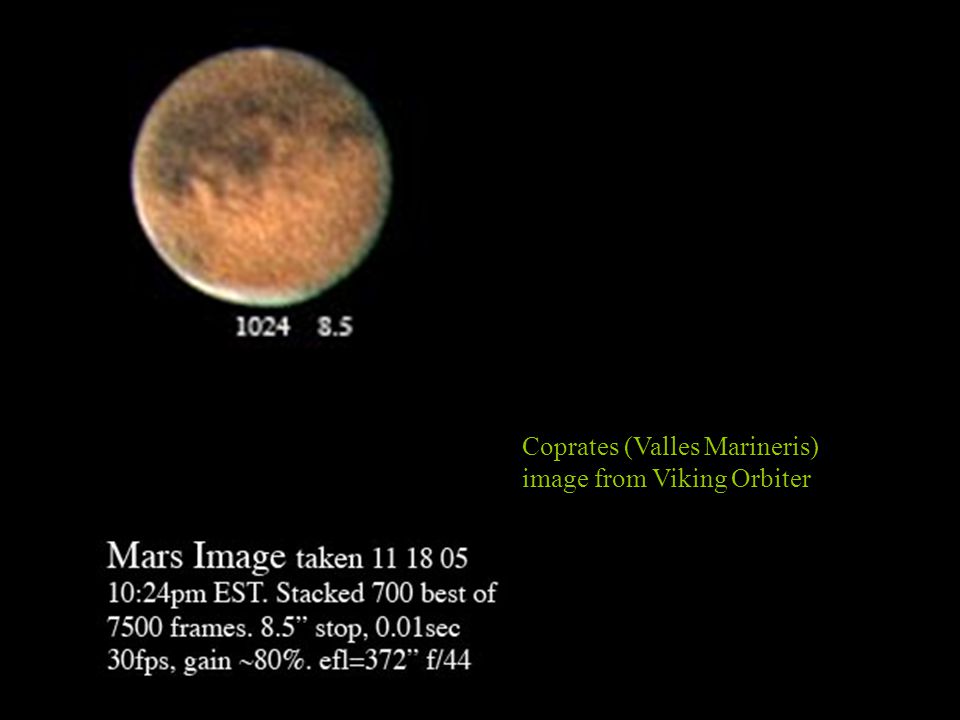
57. Coprates (Valles Marineris) image from Viking Orbiter

59. juniou Images of Jupiter showing Oval BA Red Spot Junior First Light Image taken 6/18/07 with 7.25” f/14 Schupmann using 3x Barlow lens, f/42 Seeing poor to average. Image taken 2/15/06 with 10” f/15 Refractor at Sperry Observatory using 2x Barlow lens, f/30 Seeing average.

60. That’s all, folks…

61. Helpful Hints Use a 2x Barlow for your early experiments. It gets the focus outside the drawtube and into the webcam focal plane. You might not be able to focus without it and you really need some amplification no matter how lousy the seeing is. No problem if you have an SCT. Parfocalize an eyepiece with your webcam. Life is much easier if you can prefocus before getting into the computer stuff. A motorized finder is very helpful. It is amazing how much image motion you get when you barely touch a manual focuser while you’re working at f/45. You must have a good finder. I doubt that even modern computerized GO-TO scopes are accurate enough for webcam purposes when you are using f/60 or higher. The 7-10x finder that came with your scope is probably not powerful enough. A second finder working at 25x or higher is a really good idea. I just attached a 3” f/10 Newtonian on the side of my scope with a 12.5mm illuminated eyepiece giving 60x. This works fine. Start with the moon. It is bright and easy to find and rewards you with easy good results so you don’t get discouraged. If the seeing is poor to average, don’t waste your time with full aperture if you have a 10 or 12” scope. Stop down to 5 to 8 inches.

62. Computer stuff The Computer –If you are setting up outside each time, the computer probably has to be a laptop. If you have a permanent observatory, a desktop is better. –You need a reasonably fast windows PC (no Macs, sorry), preferrably running 2000NT or XP. You can get by with ME, but it can be a painful experience. –Buy as much RAM and hard drive space as you can possibly afford, 200 gigabyte hard drive space is not too much! Get a DVD writer to use for video file backup if you can. –You need a free USB port to plug the webcam into. Webcam software: All you need is the driver and it is probably already in your system. Look for a program called VRecord using the find function in your computer. Run it after plugging your webcam into the USB port. You don’t need the stuff on the CDROM that came with your webcam. Download Registax: It’s free! http://registax.astronomy.net/ http://registax.astronomy.net/ Registax tutorials: http://www.threebuttes.com/RegistaxTutorial.htm http://www.threebuttes.com/RegistaxTutorial.htm

63. Step by Step Procedure Set up telescope and turn on drive. Turn on your computer and make sure the date and time are set correctly. Locate object in finder and insert amplifier and parfocalized eyepiece into the focuser. Center and focus object. Replace eyepiece with webcam Plug USB cable from webcam into computer. Launch VRecord. If you have centered the object properly, you will see something on the screen. It may even be in focus. If not, focus it. In the options menu, make sure that the “Set Preview” box is checked and select “Set Video Format” and verify that it is set for the default 320x240 pixel mode or whatever mode you wish to use. In file menu select “Set Capture File” and name the file appropriately for the object you are observing. I like to use the name of the object followed by the date and a serial number, such as: Mars 10 27 05 3. You don’t need to put the time information in (or even the date) since that will be timestamped on the file when it is saved after taking the video. In the capture window, select “Set Time Limit”. In the dialog box be sure to check the “Use Time Limit” box. Type in the video file length in seconds you wish to use and say ok. I use 120 or 180 seconds for planetary work and 30 seconds for lunar work where I plan to take a whole lot of pictures to make a terminator strip.

64. Step by Step Procedure, cont. In the options menu select “Video Parameters”, and under the Image Controls tab, turn off the full auto mode and select 15 frames per second and then click on the tab named “Camera Controls”. Put the exposure slider to 1/50th of a second and the gain at about 50% of full scale. If the image is too bright, select a shorter exposure, if it is too faint select a longer one or slide the gain control to a higher value. You also have controls for white level which may be difficult to use if nothing in the object is supposed to be white. Auto should be off. Make small adjustments in blue and red level until the color of the object is correct. Note: you can make these adjustments during the daytime using a distant tree top as a subject. The automatic controls will work in this case and you can let it do its thing, then turn them off and save the settings for use at night. All you will have to change at night will be the exposure or gain controls. In the capture window, select start capture. This will give you another dialog box which you have to click on again to actually start the capture. At the end of the scheduled time, the file capture will stop automatically. You don’t need to save the file since it is written to while you are taking the video. Don’t forget to create a new capture file for your next video. If you don’t, the next video will overwrite the last one and you will be very upset. When you drop the file menu and select “set capture file” again. It will come up with the name of the last file as a default. You can either type in a new name, or if you use the serial number procedure I do, just change the last number.

65. Step by Step Procedure, cont. If your computer has enough resouces (RAM, processor speed) you will able to run Registax on your.avi files as you accumulate them. If not, wait until you are done observing before trying to run Registax. I have had a number of computer crashes requiring restart because I had too many things going on at once (I was running Windows ME at the time, it is not a problem for later versions of Windows). Launch Registax. Press Select button in upper left corner of startup screen. This will give you a file browser box which will allow you to point to the one of your.avi files you wish to process. When you click on the file name (even before you click the Open button) you will see the first frame of the video in the right side of the file browser box as well as in the Registax screen behind it. If this is the correct file, press Open. When the file opens, if you move the cursor over the image you will see a square with a plus sign in the middle of it. If this square is too small (the 32 pixel one for example) processing will be fast, but the program might get lost. I like to pick the 128 pixel box when I am in the default video format of 320x240.

66. Step by Step Procedure, cont. Move the slider at the bottom of the screen to step through the video file. When you find a good frame (one that is sharper, more symmetrical, shows detail) move the cursor over the image and center the square on the object and do one left click on the mouse. At this point you will see a graph with a power spectrum of the selected frame. This is a red curve starting on the left near the top with high intensity of low spatial frequency components and dropping off rapidly to the right. You can also select a Quality Estimate method to use at this point. I really like the Gradient method. Select it if it is not already selected. You can also select the appropriate % lowest quality parameter. I would pick 80% for a start. You will also see a multicolored plot of the two dimensional Fourier transform of the image. You should see a reasonably symmetric plot with a red region in the center. If you do, you can leave it alone and press the button marked Align just below the blue tab also marked Align (if the red region is too broad, use the arrows by the FFT filter box to raise the number you see there, however, Cor’s defaults will usually work best).

67. Step by Step Procedure, cont. When you press the Align button, you will see the image area start jiggling about madly with the alignment box moving with it. This is a first pass at roughly aligning all the frames, but most importantly, it is the time when the program measures the quality of each frame by the method you selected in a previous step (use the gradient method, it works best). When the quality estimation phase is finished, you will see a graph with a red curve and a blue curve. The red one is a plot of the quality of each frame as determined by the method you chose. Registax rearrange the frame order putting the best frames to the left, the worst ones to the right. The blue curve gives you the registration difference between each frame and the reference frame you picked at the beginning. Now you get to pick how many of the best frames to keep for further processing and eventual stacking. Grab the slider at the bottom of the screen and move it to the left. The vertical green line will move to the left also. As you move it the frame number and the stack size number below slider will change. Notice that the frame numbers appear to be random now. When you have picked the stack size you wish to keep (the better the seeing, the more you get to keep) press the Limit button just below the Align button.

68. Step by Step Procedure, cont. At this point you can go on and select Optimize and Stack (or just Optimize) and the program will go through the smaller set of frames and do a better job of aligning them up with the reference frame. A better choice at this point, however, is to press the Create button. This takes the fifty best frames (or whatever number you see in the box to the right of the button) and creates a much better reference frame from them to use to do the whole set of good frames you selected. Let’s say you press the Create button. When you do, the program will rapidly optimize this small set of the best frames, stack them and give you the chance to do some processing. When it is finished you will get a redundant dialog box telling you to enhance image and press continue and you have to say OK. When you do, you can play with the wavelet sliders to perk up the image. Don’t mess around too much at this stage, otherwise the program might not recognize the unprocessed frames as being the same object as the tuned up reference frame. I would just move the slider under the checked 3:2 wavelet spot to about 50% and uncheck the first two boxes. At this point you probably are already pleased. Just wait.

69. Step by Step Procedure, cont. Press the continue button, and the redundant OK button, and then press optimize and stack. The program now goes through the rest of the good frames and optimizes their alignment very precisely against the created reference frame. When the program has finished this process, it digitally adds all the frames together, pixel by pixel to give the stacked image. You can press the preview button by each wavelet to see the contribution it will make in the final image. Some look noisy or empty. Uncheck them. When you do, the noise in that particular wavelet component of the image will be eliminated from the final image. Sort of a smart low pass filter. Some look like they have interesting detail in them. Move their sliders to higher values to see how they can help the image. A good place to start is with the first wavelet unchecked, the second one at 25%, the third and fourth at 50%, the fifth at 25% and the sixth just left alone. Play with the wavelets until you are satisfied and then you can check the box to hold the wavelet setting for processing the next video.

70. Step by Step Procedure, cont. Look closely at the image. You may see a red fringe on one side and a blue one on the other. This is atmospheric dispersion and you can tune it out! Select the RGB shift tab to the right of the screen and you will see up/down/left/right buttons for shifting both the red and the blue components of the RGB image around relative to the green one. To help you do this, you can turn off any or all of the components as well. It usually only takes a few pixels shift of the red component in one direction and a few more of the blue component in the opposite direction to make a significant improvement. The fringes should go away, and small scale details may sharpen up considerably. Now press the Final tab near the top and center of the screen. This stage of the process will allow you to rotate and or flip the image to correct for odd numbers of reflections (left and right reversed, like with a star diagonal) and make North or South up as you prefer. You now save the final image as either a bitmap or a JPEG 8 bit file, or three 16 bit formats: FITS, TIFF or PNG. The FIT option is the most accurate way to save the files as separate 16bit R, G and B components. TIFF is like jpeg and can be compressed, however it is a 16 bit file. Now press Select to load another file and start all over again. Enjoy the cool pictures!

71. Ed Grafton in Houston, Texas, imaged Mars on five successive nights from October 16 to 21 while the dust storm that began in Chryse pread southward across Mare Erythraeum and Solis Lacus. On the 21st, the dust is the wide pale- yellowish veil extending from the center partway down. Grafton used a 14’ SCT at f/39 with an SBIG ST- 402 CCD camera. North is up