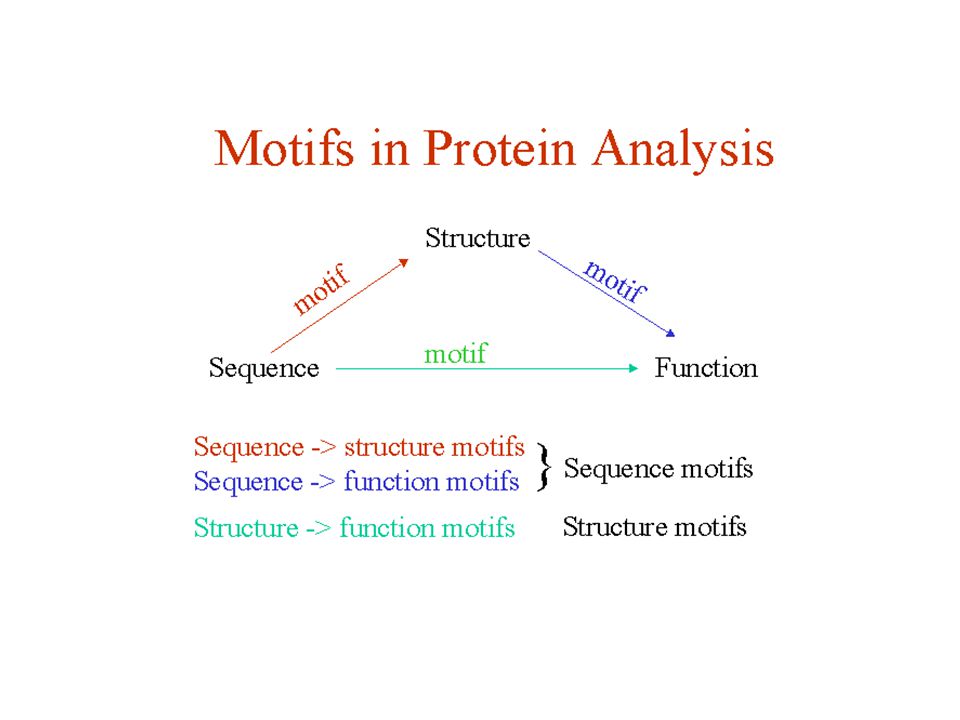
1. Introduction à la découverte de motifs en biologie moléculaire François Coste, Nov. 2005, École chercheurs BioInfo

2. Z...YLGPLNCKSCWQKFDSFSKCHDHYLCRHCLNLLL... ZFH2...ILMCFICKLSFGNVKSFSLHANTEHRLNL... ZNF236...HKCEICLLSFPKESQFQRHMRDHE... Z...YLGPLNCKSCWQKFDSFSKCHDHYLCRHCLNLLL... ZFH2...ILMCFICKLSFGNVKSFSLHANTEHRLNL... ZNF236...HKCEICLLSFPKESQFQRHMRDHE... Caractérisation d’une famille de protéines Exple : Protéines « en doigt de zinc » x x x x x x C H x \ / x x Zn x x / \ x C H x x x x x x x x x x C-x(2,4)-C-x(3)-[LIVMFYWC]-x(8)-H-x(3,5)-H

3. Motif C2H2 pour la famille Zinc finger 416 séquences Zinc finger motif C2H2 contenu dans : –372 Zinc finger –34 protéines non Zinc finger –6 protéines candidates Zinc finger C-x(2,4)-C-x(3)-[LIVMFYWC]-x(8)-H-x(3,5)-H

4. Pattern discovery overview Pattern Discovery consists to build a model (motif) of a family from a set of sequences of this family; Such a model may be either characteristic (one looks for a definition of the set of sequences) or discriminant (one looks for a difference between two sets of sequences); In all cases, the motif has a predictive value and may be checked against new sequences with a pattern matching algorithm. Pattern discovery may be applied either to nucleic or amino- acids sequences, generally with different algorithms.

5. Famille : Set de séquences ‘ reliées ’ (fonction/structure identique ) Identification d’un pattern associé à une fonction biologique - Annotation des génomes - Caractérisation de familles fonctionnelles - Recherche de nouvelles séquences Contraintes de ‘ conservation ’ sur les zones impliquées Découverte de motifs

6. Usefulness of Patterns in Genomics DNA / RNA : regulation, genes, diseases… Transcription Factors; Site of fixation of sigma factors; Regulation patterns specific of a tissue or a development stage; Transcription Terminators; Frameshift; Repeats (tandem, inverted…).

7. Usefulness of Patterns in Proteomics Proteins : Function, activity, localization, alignment… Patterns of intra-molecular links; Patterns of interaction protein/ ion, DNA, Protein; Pattern specific of tissues or addressing inside a cell; Signatures of functions Signatures of structures.

8. Specific signatures of families : comparison is not sufficient… Two situations where motifs are necessary 1.Annotation of a new sequence; 2.Search for candidates of a family of interest. In both cases, people generally use various versions of Blast. It is not the most efficient way to look at motifs since some positions are far more important than others and corresponding positions may even change from one sequence to another one. Multiple alignements, for instance with ClustalW is a better solution when possible but suffers basically from the same drawbacks.

9. Pattern discovery methods : a bench of algorithms…

10. De l’ADN aux protéines La régulation des gènes, vue par un informaticien…

11. ADN

12. De l’ADN à la fonction Code source Exécutable Compilation

13. De l’ADN à la protéine codon-start D’après Guillaume Bokiau Gène

14. Synthèse des protéines Alphabet des acides aminés : 20 lettres

15. ARN Polymérase Transcription de l’ADN en ARN

16. Ribosome Traduction de l’ARN en protéine Source : Guillaume Bokiau

17. Comment est régulée l’expression des gènes ? ARN-Polymerase : ADN → ARN ( → Protein) ADN :  30000 gènes Transcription au bon moment et au bon endroit…. Comment repérer les gènes ? Quand activer un gène ? Combien de copies ? Où ? (dans quelle cellule ?)

18. De l’ADN à la protéine codon-start D’après Guillaume Bokiau GènePromoteur

19. Gènes

20. Initiation de la transcription (procaryotes) Source Marie-France Sagot

21. Initiation de la transcription (eucaryotes) Source : Marie-France Sagot

22. TATA-Box (Pribnow-Box) : TATAAT Incluse dans : –20% des promoteurs de la levure –30% ‘’ ‘’ de l’humain D’autres types de sites de fixations : –GC-Box, CAAT-Box,… Tolérance à certaines mutations : –TATTAT fonctionnel (avec un affaiblissement potentiel du signal) –TAATAAT non fonctionnel –TATAAT présent sans mutation dans 14 des 291 TATA-Box connues…

23. Exemples de sites de fixation -150 1 2 3 4 5 6 7 8

24. Motif consensus D’après Maximilian Häußler [TCG] [ATG] [AC] C [AT] [AT] [AT] [ATC] [ATG] [AT] G G [TCG] [AC] Motif (séquence) consensus Utilisation du code IUPAC W

25. GTACATTTGAAGTA vs TAACTATAATGGGA ? D’après Maximilian Häußler Motif (séquence) consensus Utilisation du code IUPAC [TCG] [ATG] [AC] C [AT] [AT] [AT] [ATC] [ATG] [AT] G G [TCG] [AC] W A Une idée : consensus plus spécifique et permettre un nombre limité d’erreurs.

26. W Séquence consensus T A A C T A T A A T G G G A Mais: Des positions supportent mieux les mutations que d’autres… Il peut y avoir des préférences de mutations… Err 6 7 2 3 7 4 7

27. Position frequency matrix Source Maximilian Häußler

28. Probabilité d’une sous-séquence ? Exercices : Utiliser la PFM ci-dessus pour calculer : P( GTACATTTGAAGTA ) = ? P( TAACTATAATGGGA ) = ? P( AAACTATAATGGGA )= ? Comment savoir si une probabilité est significative ? Comment se comportent ces probabilités si la composition en nucléotides est biaisée ?

29. Position weights Probabilité du nucléotide b en la position i : Poids du nucléotide b en la position i (Log odds): pseudo compte background probability

30. Position weight matrix (PWM) Source Maximilian Häußler p(A)=p(T)=p(G)=p(C)=¼

31. Score d’un site Source Maximilian Häußler

32. Sequence Logo [Schneider] Source Maximilian Häußler

33. Entropie relative (information content) D’une position : D’une matrice : Mesure de la conservation du motif entre 0 et 2 bits (ADN, ¼) max = len  2 (ADN, ¼)

34. Entropie relative (information content)

38. Insertions Gap

39. A HMM model for a DNA motif alignments, The transitions are shown with arrows whose thickness indicate their probability. In each state, the histogram shows the probabilities of the four bases. « Généralisation » des PWMs

40. Consensus sequence: P (ACACATC) = 0.8x1 x 0.8x1 x 0.8x0.6 x 0.4x0.6 x 1x1 x 0.8x1 x 0.8 = 4.7 x 10 -2 To score a sequence using probability: ACAC - - ATC Probabilité de séquences

41. Highly implausible sequence: P(TGCTAGG) = 0.0023 x 10 -2 TGCT - - AGG To score a sequence using probability: Probabilité de séquences

42. To score the sequence using log-odds: log-odds for sequence S = log [P(S)/(0.25) L ] = log P(S) - L Log 0.25 Probabilities and log-odds scores for the 5 sequences in the alignment and for the consensus sequence and the exceptional sequence. Probabilité de séquences

43. Profile HMM Insertions-délétions : Match states Insert states Delete states

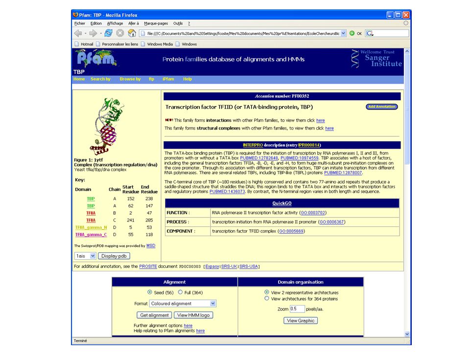
44. Séquence (format Fasta): >UniProt/Swiss-Prot|P20226|TBP_HUMAN TATA-box binding protein MDQNNSLPPYAQGLASPQGAMTPGIPIFSPMMPYGTGLTPQPIQNTNSLSILEEQQRQQQ QQQQQQQQQQQQQQQQQQQQQQQQQQQQQQQQQQQAVAAAAVQQSTSQQATQGTSGQAPQ LFHSQTLTTAPLPGTTPLYPSPMTPMTPITPATPASESSGIVPQLQNIVSTVNLGCKLDL KTIALRARNAEYNPKRFAAVIMRIREPRTTALIFSSGKMVCTGAKSEEQSRLAARKYARV VQKLGFPAKFLDFKIQNMVGSCDVKFPIRLEGLVLTHQQFSSYEPELFPGLIYRMIKPRI VLLIFVSGKVVLTGAKVRAEIYEAFENIYPILKGFRKTT Extrait du fichier PDB : P20226 Human TATA-box Binding Protein

45. Vue synthétique :

46. Interactions Lysines (K) et Arginines (R) avec les Groupes phosphates de l’ADN Pont hydrogène entre Asparagine (N) et l’ADN 2  2 Phenylalalines (F) se glissent dans le sillon de l’ADN : –interaction avec les bases –Courbure de l’ADN (flexibilité De TATA) Reconnaissance de la TATA-Box par la TATA Binding Protein

47. Other TATA-box binding proteins There are different TATA-box binding proteins that have been identified, including TBP1, TBP2, TBP3 and TBPL (TATA-box binding protein like). All of these proteins are related in terms of sequence and structure. The TBP is composed of an N-terminal that varies in both length and sequence, and a highly conserved C-terminal region that binds to the TATA box. The C-terminal region contains two 77-amino acid repeats that produce a saddle-shaped structure that straddles the DNA. In addition, the C-terminal core interacts with a variety of transcription factors as well as regulatory proteins. The N-terminal region appears to modulate DNA binding of the TBP molecule, in addition to other more specific functions.

49. Acides aminés Matrice de substitution (Blosum)

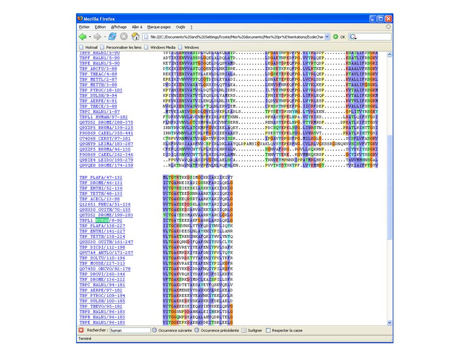
50. L’outil de découverte de motifs le plus utilisé sur les Protéines ClustalW !

52. Y-x-[PK]-x(2)-[IF]-x(2)-[LIVM](2)-x-[KRH]-x(3)-P-[RKQ]-x(3)-L-[LIVM]-F-x-

57. P20226 Human TATA-box Binding Protein Vue Interpro :

58. Banks of motifs : two general references Regulation patterns : Transfac databases of motifs for binding sites (extended with mutations, composite motifs, commercial now…) http://www.gene-regulation.com http://genouest.org Origin E. Wingenders Version 6.0 : 6627 sites http://www.gene-regulation.comhttp://genouest.org Protein patterns : A unified site for the integration of many banks : Interpro (integrates now also structural data). http://www.ebi.ac.uk/interpro/ >80% TrEMBL http://www.ebi.ac.uk/interpro/

59. Découverte de motifs

62. ClasseExemple At-c-t-t-g-a BD-R-C-C-x(2)-H-D-x-C CG-G-G-T-F-D-[ILV]-[ST]-[ILV] DV-x-P-x(2)-[RQ]-x(4)-G-x(2)-L-[LM] EG-C-x(1,3)-C-P-x(8,10)-C-C FC-x(2,4)-C-x(3)-[ILVFYC]-x(8)-H-x(3,5)-H G G-G-G-T-F-D-*- D-R-C-C-P H G-G-G-T-F-[DE]-*- D-R-C-[PAR]-C I G-G-G-x(2,5)-T-F-[DE]-*-D-x(0,1)-C-[PAR]-C J Expression régulière/Grammaire régulière/Automate K Grammaire algébrique M Grammaire contextuelle N Grammaire à structure de phrase Expressivité des motifs (Prosite, Pratt) D’après Brazma et al

63. Grammars

66. Séquences/Structures non alignées Alignement Analyse Enumération de motifs Score Motif Séquence driven Pattern driven

69. A first useful discovery method : How to discover patterns from scratch? Example of study involving a simple combinatorial search and a simple motif evaluation : RSA Tools (Jacques van Helden, Shoshana Wodak UCMB-ULB); Search of transcription sites in sequences upstream of families of genes of transcription factors in yeast. http://rsat.ulb.ac.be/rsat/

70. Hexanucleotide occurrences in the MET family Idea: Statistical test. Count hexanucleotides in the family and in the complete genome. Take as a null hypothesis a binomial law Space : 2080 patterns

71. RSA tools : Space of Hypotheses Hypotheses space : set of possible motifs. Must be chosen with biological relevance. Initial idea : motif = words of size k 4 k possibilities on DNA k=6 Size space = 4096 words But it is not possible to distinguish the DNA strands : one must rather consider pairs k=6 Size space = 2080 pairs of words

72. Test of hypotheses on sequences Assume n sequences Seq i and a word w present obs times in these sequences. The size of the space of word hypotheses is NH. The probability Pw of w is estimated by the frequency on a set of non coding regions of the genome at hand (or a close genome, or…). Max number of words of size w (2 strands) The significativity score is simply - log 10 ( E-value)

73. Results for MET family Known patternFactors TCACGTGCbf1p/Met4p/Met28p AAAACTGTGGMet31p; Met32p

74. A case that does not work so well... family GAL (genes expressed in presence of galactose): not even a single significant pattern !

75. Structure of the interface Gal4p-ADN

76. Solution : introduction of a gap in the pattern, between 0 and 16 Space : 35360 or 1632 if one takes into account only repeats or palindromes Pb : the method is not general enough…

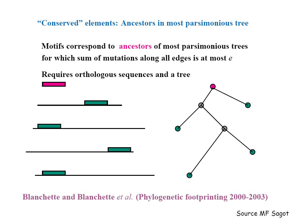
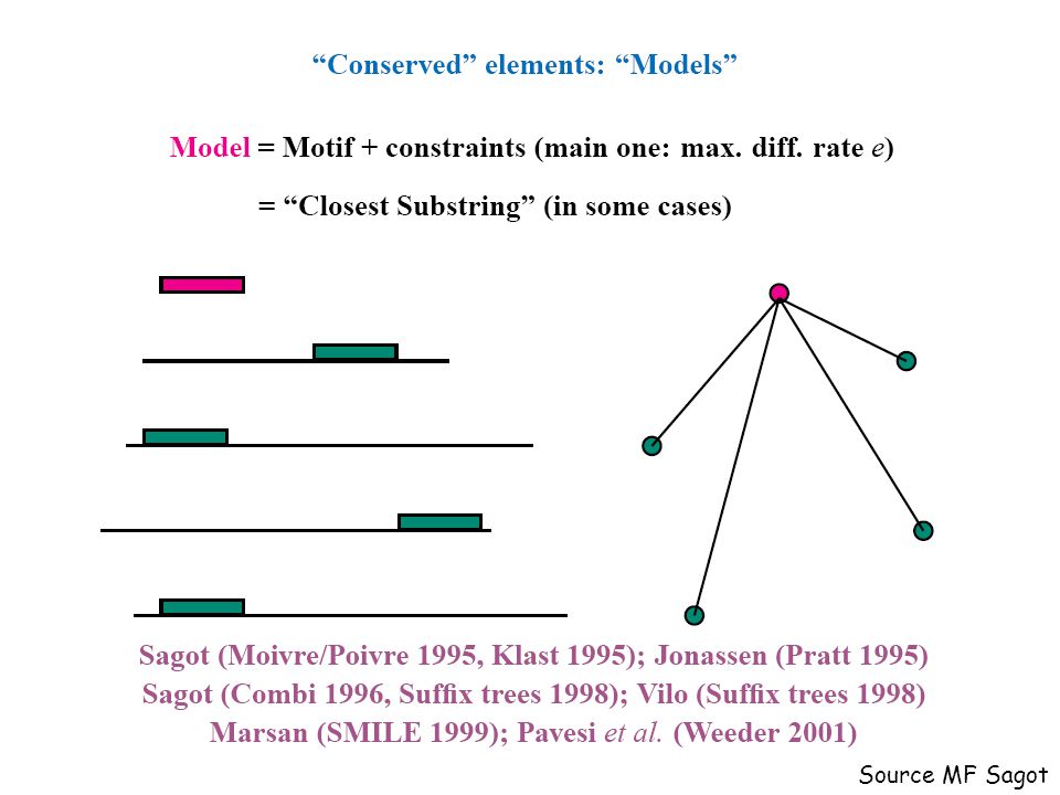
77. Source MF Sagot

89. Smile [Marsan et Sagot 2000] Recherche exacte des mots présents : dans au moins q séquences (quorum) avec au plus e erreurs Un exemple de recherche combinatoire de motifs consensus

90. Source Laurent Marsan

91. Structure de données Source Laurent Marsan

92. Structure de données Source Laurent Marsan

93. Algorithme de base Source Laurent Marsan

96. Arrêt de la descente récursive Source Laurent Marsan

97. Dyades Source Laurent Marsan

105. Source MF Sagot

108. Heuristiques Expectation-Maximization –MEME, Bailey, 1995 Gibbs Sampling –Lawrence et al, 1993 –Thijs et al, 2001 Algorithme glouton –(w)consensus, Hertz et al, 1999 Projection –Buhler et al, 2000

109. Simplified Principle of deterministic algorithm EM Initialization : For all sequences, select at random a site (window of size k). Do –« Expectation » Compute on the set of sites of sequences a model M from the frequency matrix (letters x positions). –« Maximization » For each sequence Compute a likelihood score for each site (window of size k), based on its probability with respect to M and the Background (vector estimated on a larger sample). Select the site of best likelihood score for the sequence Until stability of model M M ( Used in MM of MEME ) Words of size k

110. Gibbs Sampling Source: Jun Liu

111. Gibbs Sampling (cont’d) Source: Jun Liu

112. Gibbs Sampling Example The following slides illustrate Gibbs sampling to discover a motif in yeast DNA sequences. This example uses a sequence model that allows multiple sites per sequence. Columns are sampled as well as sites.

113. 5’- TCTCTCTCCACGGCTAATTAGGTGATCATGAAAAAATGAAAAATTCATGAGAAAAGAGTCAGACATCGAAACATACAT 5’- ATGGCAGAATCACTTTAAAACGTGGCCCCACCCGCTGCACCCTGTGCATTTTGTACGTTACTGCGAAATGACTCAACG 5’- CACATCCAACGAATCACCTCACCGTTATCGTGACTCACTTTCTTTCGCATCGCCGAAGTGCCATAAAAAATATTTTTT 5’- TGCGAACAAAAGAGTCATTACAACGAGGAAATAGAAGAAAATGAAAAATTTTCGACAAAATGTATAGTCATTTCTATC 5’- ACAAAGGTACCTTCCTGGCCAATCTCACAGATTTAATATAGTAAATTGTCATGCATATGACTCATCCCGAACATGAAA 5’- ATTGATTGACTCATTTTCCTCTGACTACTACCAGTTCAAAATGTTAGAGAAAAATAGAAAAGCAGAAAAAATAAATAA 5’- GGCGCCACAGTCCGCGTTTGGTTATCCGGCTGACTCATTCTGACTCTTTTTTGGAAAGTGTGGCATGTGCTTCACACA …HIS7 …ARO4 …ILV6 …THR4 …ARO1 …HOM2 …PRO3 300-600 bp of upstream sequence per gene are searched in Saccharomyces cerevisiae. The Input Data Set Source: G.M. Church

114. 5’- TCTCTCTCCACGGCTAATTAGGTGATCATGAAAAAATGAAAAATTCATGAGAAAAGAGTCAGACATCGAAACATACAT 5’- ATGGCAGAATCACTTTAAAACGTGGCCCCACCCGCTGCACCCTGTGCATTTTGTACGTTACTGCGAAATGACTCAACG 5’- CACATCCAACGAATCACCTCACCGTTATCGTGACTCACTTTCTTTCGCATCGCCGAAGTGCCATAAAAAATATTTTTT 5’- TGCGAACAAAAGAGTCATTACAACGAGGAAATAGAAGAAAATGAAAAATTTTCGACAAAATGTATAGTCATTTCTATC 5’- ACAAAGGTACCTTCCTGGCCAATCTCACAGATTTAATATAGTAAATTGTCATGCATATGACTCATCCCGAACATGAAA 5’- ATTGATTGACTCATTTTCCTCTGACTACTACCAGTTCAAAATGTTAGAGAAAAATAGAAAAGCAGAAAAAATAAATAA 5’- GGCGCCACAGTCCGCGTTTGGTTATCCGGCTGACTCATTCTGACTCTTTTTTGGAAAGTGTGGCATGTGCTTCACACA AAAAGAGTCA AAATGACTCA AAGTGAGTCA AAAAGAGTCA GGATGAGTCA AAATGAGTCA GAATGAGTCA AAAAGAGTCA ********** MAP score = 20.37 (maximum) …HIS7 …ARO4 …ILV6 …THR4 …ARO1 …HOM2 …PRO3 The Target Motif Source: G.M. Church

115. 5’- TCTCTCTCCACGGCTAATTAGGTGATCATGAAAAAATGAAAAATTCATGAGAAAAGAGTCAGACATCGAAACATACAT 5’- ATGGCAGAATCACTTTAAAACGTGGCCCCACCCGCTGCACCCTGTGCATTTTGTACGTTACTGCGAAATGACTCAACG 5’- CACATCCAACGAATCACCTCACCGTTATCGTGACTCACTTTCTTTCGCATCGCCGAAGTGCCATAAAAAATATTTTTT 5’- TGCGAACAAAAGAGTCATTACAACGAGGAAATAGAAGAAAATGAAAAATTTTCGACAAAATGTATAGTCATTTCTATC 5’- ACAAAGGTACCTTCCTGGCCAATCTCACAGATTTAATATAGTAAATTGTCATGCATATGACTCATCCCGAACATGAAA 5’- ATTGATTGACTCATTTTCCTCTGACTACTACCAGTTCAAAATGTTAGAGAAAAATAGAAAAGCAGAAAAAATAAATAA ********** TGAAAAATTC GACATCGAAA GCACTTCGGC GAGTCATTAC GTAAATTGTC CCACAGTCCG TGTGAAGCAC 5’- TCTCTCTCCACGGCTAATTAGGTGATCATGAAAAAATGAAAAATTCATGAGAAAAGAGTCAGACATCGAAACATACAT 5’- ATGGCAGAATCACTTTAAAACGTGGCCCCACCCGCTGCACCCTGTGCATTTTGTACGTTACTGCGAAATGACTCAACG 5’- CACATCCAACGAATCACCTCACCGTTATCGTGACTCACTTTCTTTCGCATCGCCGAAGTGCCATAAAAAATATTTTTT 5’- TGCGAACAAAAGAGTCATTACAACGAGGAAATAGAAGAAAATGAAAAATTTTCGACAAAATGTATAGTCATTTCTATC 5’- GGCGCCACAGTCCGCGTTTGGTTATCCGGCTGACTCATTCTGACTCTTTTTTGGAAAGTGTGGCATGTGCTTCACACA ********** TGAAAAATTC GACATCGAAA GCACTTCGGC GAGTCATTAC GTAAATTGTC CCACAGTCCG TGTGAAGCAC MAP score = -10.0 …HIS7 …ARO4 …ILV6 …THR4 …ARO1 …HOM2 …PRO3 Initial Seeding Source: G.M. Church

116. 5’- TCTCTCTCCACGGCTAATTAGGTGATCATGAAAAAATGAAAAATTCATGAGAAAAGAGTCAGACATCGAAACATACAT 5’- ATGGCAGAATCACTTTAAAACGTGGCCCCACCCGCTGCACCCTGTGCATTTTGTACGTTACTGCGAAATGACTCAACG 5’- CACATCCAACGAATCACCTCACCGTTATCGTGACTCACTTTCTTTCGCATCGCCGAAGTGCCATAAAAAATATTTTTT 5’- TGCGAACAAAAGAGTCATTACAACGAGGAAATAGAAGAAAATGAAAAATTTTCGACAAAATGTATAGTCATTTCTATC 5’- ACAAAGGTACCTTCCTGGCCAATCTCACAGATTTAATATAGTAAATTGTCATGCATATGACTCATCCCGAACATGAAA 5’- ATTGATTGACTCATTTTCCTCTGACTACTACCAGTTCAAAATGTTAGAGAAAAATAGAAAAGCAGAAAAAATAAATAA 5’- GGCGCCACAGTCCGCGTTTGGTTATCCGGCTGACTCATTCTGACTCTTTTTTGGAAAGTGTGGCATGTGCTTCACACA ********** TGAAAAATTC GACATCGAAA GCACTTCGGC GAGTCATTAC GTAAATTGTC CCACAGTCCG TGTGAAGCAC Add? ********** TGAAAAATTC GACATCGAAA GCACTTCGGC GAGTCATTAC GTAAATTGTC CCACAGTCCG TGTGAAGCAC TCTCTCTCCA How much better is the alignment with this site as opposed to without? …HIS7 …ARO4 …ILV6 …THR4 …ARO1 …HOM2 …PRO3Sampling Source: G.M. Church

117. 5’- TCTCTCTCCACGGCTAATTAGGTGATCATGAAAAAATGAAAAATTCATGAGAAAAGAGTCAGACATCGAAACATACAT 5’- ATGGCAGAATCACTTTAAAACGTGGCCCCACCCGCTGCACCCTGTGCATTTTGTACGTTACTGCGAAATGACTCAACG 5’- CACATCCAACGAATCACCTCACCGTTATCGTGACTCACTTTCTTTCGCATCGCCGAAGTGCCATAAAAAATATTTTTT 5’- TGCGAACAAAAGAGTCATTACAACGAGGAAATAGAAGAAAATGAAAAATTTTCGACAAAATGTATAGTCATTTCTATC 5’- ACAAAGGTACCTTCCTGGCCAATCTCACAGATTTAATATAGTAAATTGTCATGCATATGACTCATCCCGAACATGAAA 5’- ATTGATTGACTCATTTTCCTCTGACTACTACCAGTTCAAAATGTTAGAGAAAAATAGAAAAGCAGAAAAAATAAATAA 5’- GGCGCCACAGTCCGCGTTTGGTTATCCGGCTGACTCATTCTGACTCTTTTTTGGAAAGTGTGGCATGTGCTTCACACA ********** TGAAAAATTC GACATCGAAA GCACTTCGGC GAGTCATTAC GTAAATTGTC CCACAGTCCG TGTGAAGCAC Add? ********** TGAAAAATTC GACATCGAAA GCACTTCGGC GAGTCATTAC GTAAATTGTC CCACAGTCCG TGTGAAGCAC How much better is the alignment with this site as opposed to without? Remove. ATGAAAAAAT …HIS7 …ARO4 …ILV6 …THR4 …ARO1 …HOM2 …PRO3 Continued Sampling Source: G.M. Church

118. 5’- TCTCTCTCCACGGCTAATTAGGTGATCATGAAAAAATGAAAAATTCATGAGAAAAGAGTCAGACATCGAAACATACAT 5’- ATGGCAGAATCACTTTAAAACGTGGCCCCACCCGCTGCACCCTGTGCATTTTGTACGTTACTGCGAAATGACTCAACG 5’- CACATCCAACGAATCACCTCACCGTTATCGTGACTCACTTTCTTTCGCATCGCCGAAGTGCCATAAAAAATATTTTTT 5’- TGCGAACAAAAGAGTCATTACAACGAGGAAATAGAAGAAAATGAAAAATTTTCGACAAAATGTATAGTCATTTCTATC 5’- ACAAAGGTACCTTCCTGGCCAATCTCACAGATTTAATATAGTAAATTGTCATGCATATGACTCATCCCGAACATGAAA 5’- ATTGATTGACTCATTTTCCTCTGACTACTACCAGTTCAAAATGTTAGAGAAAAATAGAAAAGCAGAAAAAATAAATAA 5’- GGCGCCACAGTCCGCGTTTGGTTATCCGGCTGACTCATTCTGACTCTTTTTTGGAAAGTGTGGCATGTGCTTCACACA ********** GACATCGAAA GCACTTCGGC GAGTCATTAC GTAAATTGTC CCACAGTCCG TGTGAAGCAC Add? ********** TGAAAAATTC GACATCGAAA GCACTTCGGC GAGTCATTAC GTAAATTGTC CCACAGTCCG TGTGAAGCAC How much better is the alignment with this site as opposed to without? …HIS7 …ARO4 …ILV6 …THR4 …ARO1 …HOM2 …PRO3 Continued Sampling Source: G.M. Church

119. 5’- TCTCTCTCCACGGCTAATTAGGTGATCATGAAAAAATGAAAAATTCATGAGAAAAGAGTCAGACATCGAAACATACAT 5’- ATGGCAGAATCACTTTAAAACGTGGCCCCACCCGCTGCACCCTGTGCATTTTGTACGTTACTGCGAAATGACTCAACG 5’- CACATCCAACGAATCACCTCACCGTTATCGTGACTCACTTTCTTTCGCATCGCCGAAGTGCCATAAAAAATATTTTTT 5’- TGCGAACAAAAGAGTCATTACAACGAGGAAATAGAAGAAAATGAAAAATTTTCGACAAAATGTATAGTCATTTCTATC 5’- ACAAAGGTACCTTCCTGGCCAATCTCACAGATTTAATATAGTAAATTGTCATGCATATGACTCATCCCGAACATGAAA 5’- ATTGATTGACTCATTTTCCTCTGACTACTACCAGTTCAAAATGTTAGAGAAAAATAGAAAAGCAGAAAAAATAAATAA 5’- GGCGCCACAGTCCGCGTTTGGTTATCCGGCTGACTCATTCTGACTCTTTTTTGGAAAGTGTGGCATGTGCTTCACACA ********** GACATCGAAA GCACTTCGGC GAGTCATTAC GTAAATTGTC CCACAGTCCG TGTGAAGCAC ********* * GACATCGAAAC GCACTTCGGCG GAGTCATTACA GTAAATTGTCA CCACAGTCCGC TGTGAAGCACA How much better is the alignment with this new column structure? …HIS7 …ARO4 …ILV6 …THR4 …ARO1 …HOM2 …PRO3 Column Sampling Source: G.M. Church

120. 5’- TCTCTCTCCACGGCTAATTAGGTGATCATGAAAAAATGAAAAATTCATGAGAAAAGAGTCAGACATCGAAACATACAT 5’- ATGGCAGAATCACTTTAAAACGTGGCCCCACCCGCTGCACCCTGTGCATTTTGTACGTTACTGCGAAATGACTCAACG 5’- CACATCCAACGAATCACCTCACCGTTATCGTGACTCACTTTCTTTCGCATCGCCGAAGTGCCATAAAAAATATTTTTT 5’- TGCGAACAAAAGAGTCATTACAACGAGGAAATAGAAGAAAATGAAAAATTTTCGACAAAATGTATAGTCATTTCTATC 5’- ACAAAGGTACCTTCCTGGCCAATCTCACAGATTTAATATAGTAAATTGTCATGCATATGACTCATCCCGAACATGAAA 5’- ATTGATTGACTCATTTTCCTCTGACTACTACCAGTTCAAAATGTTAGAGAAAAATAGAAAAGCAGAAAAAATAAATAA 5’- GGCGCCACAGTCCGCGTTTGGTTATCCGGCTGACTCATTCTGACTCTTTTTTGGAAAGTGTGGCATGTGCTTCACACA AAAAGAGTCA AAATGACTCA AAGTGAGTCA AAAAGAGTCA GGATGAGTCA AAATGAGTCA GAATGAGTCA AAAAGAGTCA ********** MAP score = 20.37 …HIS7 …ARO4 …ILV6 …THR4 …ARO1 …HOM2 …PRO3 The Best Motif Source: G.M. Church

121. Profile HMMs: were introduced into computational biology in the late 1980’s, and for use as profile models since 1994. Profile HMMs and HMM-based genefinders are the most successful HMM applications in computational biology. Profile HMM

122. A small profile HMM (right) representing a short multiple alignment of five sequences (left) with three consensus columns. Profile HMM

123. Dynamic HMM algorithms: Forward (for scoring) and Viterbi (for alignment) were used. They have a worst case of O(NM 2 ) in time and O(NM) in space for a sequence of length N and an HMM of M states. For profile HMMs: that have a constant number of state transitions per state rather than the vector of M transitions per state in fully connected HMMs, both algorithms run in O(NM) in time and O(NM) in space. Des HMM simplifiés

124. Parameters set: an HMM can be built from prealigned (prelabeled) sequences (i.e, where the state paths are assumed to be known). It’s simply a matter of converting observed counts of symbol emissions and state transitions into probabilities. In building a profile HMM, an existing multiple alignment is given as input. HMM training algorithms: BaumWelch expectation maximization or gradient descent algorithms. Gibbs sampling, simulated annealing and genetic algorithm training methods seem better at avoiding spurious local optima in training HMMs and HMM like models. Entraînement

125. The primary advantage of these models over standard methods of sequence search is their ability to characterize an entire family of sequences. Thus, each position has a distribution of amino acid, as do transitions between states. That is, these linear HMMs have position-dependent character distributions and position-dependent insertion and deletion gap penalties. The alignment of each of a family to a trained model automatically yields a multiple alignment among those sequences.

126. An alignment of 30 short amino acid sequences chopped out of a alignment of the SH3 domain. The shaded area are the most conserved and were represented by the main states in the HMM. The unshaded area was represented by an insert state.SH3 domain Building Profile HMM

127. Note: transition lines with no arrow head are from left to right. Transitions with probability zero are not shown, and those with very small probability are shown as dashed lines. Transitions from an insert state to itself are not shown; instead the probability times 100 is shown in the diamond. The numbers in the circular delete states are just position numbers. (from SAM package of programs) Result

128. Pseudocounts Adding one to all the counts can be interpreted as assuming a priori that all the amino acids are equally likely. However, there are significant differences in the occurrence of the 20 amino acids in known protein sequences. Therefore, the next step is to use pseudocounts proportional to the observed frequencies of the amino acids instead. This is the minimum level of pseudocounts to be used in any real application of HMMs. Because a column in the alignment may contain information about the preferred type of amino acids, it is also possible to use more sophisticated pseudocount strategies. If a column consists predominantly of leucine (as above), one would expect substitutions to other hydrophobic amino acids to be more probable than substitutions to hydrophilic amino acids. One can e.g. derive pseudocounts for a given column from substitution matrices. See also SAM Tutorial…

129. Result + pseudocounts

130. A partir d’une seule séquence

131. The difference between these software packages is the model architecture they adopt: “profile” models & “motif” models. Motif model architecture: modeling one or more ungapped blocks of sequence consensus separated by a small number of insert states. Can be viewed as special cases of profile HMMs. Logiciels

132. Profile model architecture: models with an insert and delete state associated with each match state, allowing insertion and deletion anywhere in a target sequence. Logiciels

133. Three principal advances on Profile HMM methods: 1. Motif based HMMs have been introduced as an alternative to the original Krogh profile HMM architecture. 2. Large libraries of profile HMMs and multiple alignments have become available, as well as compute servers to search query sequences against these resources. 3. There has been an increasing incursion of profile HMM methods into the area of protein structure prediction by fold recognition. Conclusions (PHMM) Profile HMM method is a complement to BLAST and FASTA analyses It will provide a second tier of solid, sensitive, statistically based analysis tools, based on the combination of powerful new HMM software and large sequence alignment databases of conserved protein domains.

134. Découverte de motifs expressifs sur les protéines Pratt

135. An example of combinatorial method Aim generally at finding an expression, i.e. a pattern belonging to a language that is user-restricted with various parameters; For this purpose, explore the space of possible patterns in an ordered way, following the degree of generality (covering degree) and a fitness score. Pratt : Inge Jonassen 1996, program easily available, good expressivity.

136. Pratt’s patterns C-x(3)-[ILVFYC]-D-x(8)-H-x(3,5)-H Limitations : PMaximum Number of components L Maximum Length of a pattern : p+  j k W Maximum Length of a Wild-card F Maximum Flexibility of a Flexible Wild-card : (j-i) N Maximum Number of Flexible Wild-cards FPMaximum Value of the product of flexibilities :  (j k -i k +1) ) Pattern « PROSITE » : A 1 [x(i k,j k ) Ak], k=2,p Identity Component Ambiguous Component Fixed Wild-card x(i) Flexible Wild-card x(i,j) 5 23 8 2 6

137. Principes Pattern Driven basé sur Jonassen et al. 1995 Partir d’un petit motif (un acide aminé) et l’étendre (avec d ’autres acides aminés) tant que l’on respecte les limites de complexité choisies (longueur du motif, nombre de wildcards, …)

138. Principes (2) On peut distinguer l’utilisation pratique de deux types d’approches –Bottom-up trouver des motifs par extension de motifs plus petits –Top-down trouver des motifs par intersection entre séquences

139. Principe (3) BU Arbre de recherche de l’espace des solutions NP (-) A C D E … N … Y NPA NPC NPE … NPN NPAx NPAxT

140. Algorithme combinant BU et TD Utilisation de l’approche Bottom-up pour faire émerger des motifs candidats Positionnement des candidats sur les séquences Alignement des séquences par rapport à ces candidats (points d’ancrage) Extension à gauche et à droite et évaluation des scores des nouveaux candidats de manière à poursuivre s’il y a augmentation

141. Points d ’ancrage La version 1 de Pratt permet d’orienter la recherche en fonction de Blocks (petits alignements locaux sans gaps de sous- séquences de même taille) La version 2 permet de restreindre les motifs à ceux qui valident les séquences tout en respectant un alignement multiple

142. Paramètres utilisés dans Pratt Nombreux paramètres pour définir l’espace de recherche Paramètres pour orienter la stratégie de recherche –Compromis complexité/exhaustivité –Utilisation d’un alignement ou d’une séquence imposée. Paramètre de choix du score –Quantité d’information –MDL (Minimum Description Length)

143. Pratt’s algorithm (v2) Construction of a pattern graph of allowed patterns ; Patterns:={(  0,Root  }; While Patterns  #initial search# do For each (P,Score,Node) in Patterns #initial search# do LQ:= add_one_edge(P,Node); LQ’:=Generalize2or3(P); For each Q’ in LQ’ If Q covers at least M instances Then Patterns := Patterns  {(Q’, score(Q’))} Patterns:= Sort_H_best_scores(Patterns); While Patterns  #refinment# do For each P in Patterns LQ:=Specialize _with_ambiguity(P); R:=  ; For each Q in LQ If Q covers at least M instances Then Patterns := Patterns  {(Q, score(Q))} Patterns:= Sort_H_best_scores(Patterns)

144. Pratt Ouest Genopole

145. Doigts de Zinc : paramètres Pratt

146. Doigts de Zinc : motifs Pratt

147. Résultats avancés de Pratt sur les doigts de Zinc

148. Vue graphique des occurrences dans les séquences de doigts de Zinc

149. BONSAI [1] A Machine Discovery from Amino Acid Sequences by Decision Trees over Regular Patterns, S. Arikawa, S. Kuhara, Y Mukouchi, T. Shinohara New Generation Computing, pp 361-375, 1993 [2] Knowledge Acquisition from Amino Acid Sequences by Machine Learning System BONSAI, S. Shimozono, A. Shinohara, T. Shinohara, S. Miyano, S. Kuhara, S. Arikawa Transactions of Information Processing Society of Japan, 1994 [3] BONSAI Garden: Parallel Knowledge Discovery System for Amino Acid Sequences, International Conference on Intelligent System for Molecular Biology (ISMB’95), T. Shoudai, M.Lappe, S. Miyano, A. Shinohara, T. Okazaki, S. Arikawa, T. Uchida, S.Shimozono, T.Shinohara, S.Kuhara http://www.i.kyushu-u.ac.jp/~shoudai/papers/BONSAI-Garden.html http://www.i.kyushu-u.ac.jp/~shoudai/papers/BONSAI-Garden.html http://bonsai.ims.u-tokyo.ac.jp/services/services.htmlhttp://bonsai.ims.u-tokyo.ac.jp/services/services.html (« soon »)

150. Vue générale de BONSAI Exemples et contre exemples (tirés des Bases de Données) Séparation en échantillon d’apprentissage et de validation Recodage Apprentissage et évaluation

151. Exemple : prédiction de domaines transmembranaires

152. Construction de l’arbre de décision

153. Choix de l’attribut cf. critère ID3 Énumération exhaustive des mots  présents dans P et N et choix de celui minimisant E( ,P,N):

154. Recodage (Alphabet indexing) Trouver  :  tq  (P)   (N) =  est un problème NP-Complet Heuristique de recherche locale : 1. Choix aléatoire de  2. Pour chaque voisin  ’ de  Évaluer le score de  ’ (score de l’arbre de décision) 3. Si meilleur score,  meilleur(  ’) et aller en 2. Sinon retourner  Approximation en temps polynomial [Shimonozo 1995] ? Cluster analysis [Nakakuni et al 1994] ? Expérimentations algos génétiques  trop long.

155. Bonsai Garden Proposition de plusieurs solutions –Bruit –Sous classes Parallélisme (avec un jardinier…)

156. Bonsai Garden Prédiction de promoteurs CCAAT, GC et TATA box

157. BONSAI Garden Prédiction hélices 

158. Utilisation de motifs plus expressifs A Practical Algorithm to Find the Best Subsequence Patterns Masahiro Hirao, Hiromasa Hoshino, Ayumi Shinohara, Masayuki Takeda, Setsuo Arikawa, DS 2000 et TCS2003 A Practical Algorithm to Find the Best Episode Patterns Masahiro Hirao, Shunsuke Inenaga, Ayumi Shinohara, Masayuki Takeda, Setsuo Arikawa DS 2001 Discovering best Variable-Length-Don’t-Care Pattern Shunsuke Inenaga, Hideo Bannai, Ayumi Shinohara, Masayuki Takeda, and Setsuo Arikawa DS 2002 Transparents de l’exposé disponible sur la page de Shunsuke Inenaga

159. Subsequence Pattern Sous mot (subsequence) v de w: mot inclus dans w (en respectant l’ordre) Exple :w = abbaaabaab v = bbba –i.e. v peut être obtenu à partir de w en effaçant certaines lettres –i.e. en utilisant  pour désigner n’importe quel mot ( Variable-Length-Don’t-Care (VLDC)) : w =  v 1  v 2  …  v m  VLDC pattern  (    ) *  bb  ba  VLDC subsequence pattern   (   ) *  b  b  b  a 

160. Discovery Science 2002 Lubeck, Germany, 11.23.2002 Discovering Best Variable-Length-Don’t-Care Patterns S. Inenaga et al... FindBestVLDC(S, T) bestScore =  ; bestVLDC =  ; For all possible pattern p do x p = numOfMatchedStr(p, S); y p = numOfMatchedStr(p, T); score = f(x p, y p, |S|, |T|); if score > bestScore then bestScore = score; bestSubseq = p; return bestVLDC; computing the “goodness” of pattern p Basic Algorithm speed-up of these parts reduce patterns for candidates Source S. Inenaga

161. Discovery Science 2002 Lubeck, Germany, 11.23.2002 Discovering Best Variable-Length-Don’t-Care Patterns S. Inenaga et al... Prune the Search Tree – the first key - a b  ………………….. Cut!!  = {a, b} = {a, b} The search space is exponential… Source S. Inenaga

162. Discovery Science 2002 Lubeck, Germany, 11.23.2002 Discovering Best Variable-Length-Don’t-Care Patterns S. Inenaga et al... Score Function The “goodness” of pattern p good(p, S, T) = f(x p, y p, |S|, |T|) S, T : given sets of strings x p : num. of strings in S that p matches y p : num. of strings in T that p matches conic Chi2, Gain d’information, Gini sont coniques Source S. Inenaga

163. Discovery Science 2002 Lubeck, Germany, 11.23.2002 Discovering Best Variable-Length-Don’t-Care Patterns S. Inenaga et al... for any 0  y  y max, there exists some x 1 such that – f(x, y)  f(x’, y) for any 0  x < x’  x 1 – f(x, y)  f(x’, y) for any x 1  x < x’  x max f(x, y)  f(x’, y) non-increasing for any 0  x  x max, there exists some y 1 such that – f(x, y)  f(x, y’) for any 0  y < y’  y 1 – f(x, y)  f(x, y’) for any y 1  y < y’  y max Conic Function Function f(x, y) is conic if Source S. Inenaga

164. Discovery Science 2002 Lubeck, Germany, 11.23.2002 Discovering Best Variable-Length-Don’t-Care Patterns S. Inenaga et al... for any 0  y  y max, there exists some x 1 such that – f(x, y)  f(x’, y) for any 0  x < x’  x 1 – f(x, y)  f(x’, y) for any x 1  x < x’  x max f(x, y)  f(x’, y) non-decreasing for any 0  x  x max, there exists some y 1 such that – f(x, y)  f(x, y’) for any 0  y < y’  y 1 – f(x, y)  f(x, y’) for any y 1  y < y’  y max Conic Function (Cont.) Function f(x, y) is conic if Source S. Inenaga

165. Discovery Science 2002 Lubeck, Germany, 11.23.2002 Discovering Best Variable-Length-Don’t-Care Patterns S. Inenaga et al... x y x y x f x f Conic Function (Cont.) Source S. Inenaga

166. Discovery Science 2002 Lubeck, Germany, 11.23.2002 Discovering Best Variable-Length-Don’t-Care Patterns S. Inenaga et al... Conic Function (Cont.) x y x y y f y f Source S. Inenaga

167. Discovery Science 2002 Lubeck, Germany, 11.23.2002 Discovering Best Variable-Length-Don’t-Care Patterns S. Inenaga et al... Property of Conic Function (x, y) (0, y) (x, 0) (0, 0) (x’, y’) = max{f(0, 0), f(x, 0), f(0, y), f(x, y)} f(x’, y’)  upperBound(x, y) upperBound(x, y) : the maximum value on the square Source S. Inenaga

168. Discovery Science 2002 Lubeck, Germany, 11.23.2002 Discovering Best Variable-Length-Don’t-Care Patterns S. Inenaga et al... Pruning Heuristics numOfMatchedStr(p, S) numOfMatchedStr(p, T) d  sco d  scover < The current best score  The goodness of d  scover The upperBound of d  sco

169. Discovery Science 2002 Lubeck, Germany, 11.23.2002 Discovering Best Variable-Length-Don’t-Care Patterns S. Inenaga et al... FindBestVLDC(S, T) bestScore =  ; bestVLDC =  ; For all possible pattern p do x p = numOfMatchedStr(p, S); y p = numOfMatchedStr(p, T); score = f(x p, y p, |S|, |T|); if score > bestScore then bestScore = score; bestSubseq = p; return bestVLDC; computing the “goodness” of pattern p Basic Algorithm speed-up of these parts Source S. Inenaga

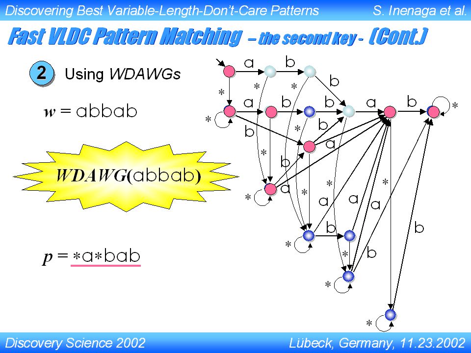
170. Discovery Science 2002 Lubeck, Germany, 11.23.2002 Discovering Best Variable-Length-Don’t-Care Patterns S. Inenaga et al... Fast VLDC Pattern Matching – the second key - 1 2 Using DFA for VLDC patterns Using Wildcard Directed Acyclic Word Graphs for text strings Pattern Matching Machine Index Structure Source S. Inenaga

171. Discovery Science 2002 Lubeck, Germany, 11.23.2002 Discovering Best Variable-Length-Don’t-Care Patterns S. Inenaga et al... abab  -{ a }  -{ b }  -{ a, b }  -{ b }  b Computing the Minimum Window Size (Cont.) Using DFA for VLDC patterns1 p =  a  bab  w = aabbab Source S. Inenaga

174. La suite… ARN : plutôt motifs structuraux « Junk » DNA Protéines, prise en compte du repliement de la protéine (motifs 3D) Prise en compte des dépendances entre positions, enchaînement des motifs… Apprentissage « croisé » avec : –données d’expressions, –génomique comparative, –topologie des protéines, –…

175. Quelques références bibliographiques générales… Motif Discovery on Promoter Sequences, Maximilian Haußler, Jacques Nicolas, 2005 An Introduction to Hidden Markov Models for Biological Sequences, A. Krogh, 1998 Finding Patterns in Biological Sequences, Brejová et al, 2000

176. Pour pratiquer RSA tools Packages HMM Plate-forme découverte de motifs Ouest Genopole

177. Oups trop loin !