1. Exemples instructifs… Représentations graphiques

2. Fonctions de répartition x=1:6 y=rep(1/6,6) z=cumsum(y) plot(c(0,x),c(0,z),lwd=3,col="blue") segments(0,0,1,0,col="green") segments(x,z, x+1,z)

3. Utiliser des données de packages existants search() [1] ".GlobalEnv" "package:methods" "package:stats" [4] "package:graphics" "package:grDevices" "package:utils" [7] "package:datasets" "Autoloads" "package:base" library( ) ash David Scott's ASH routines base The R Base Package boot Bootstrap R (S-Plus) Functions (Canty) class Functions for Classification cluster Functions for clustering (by Rousseeuw et al.)…… MASS Main Package of Venables and Ripley's MASS……

4. library(MASS);search() [1] ".GlobalEnv" "package:MASS" "package:methods" [4] "package:stats" "package:graphics" "package:grDevices" [7] "package:utils" "package:datasets" "Autoloads" [10] "package:base" data(iris); iris Sepal.Length Sepal.Width Petal.Length Petal.Width Species 1 5.1 3.5 1.4 0.2 setosa 2 4.9 3.0 1.4 0.2 setosa 3 4.7 3.2 1.3 0.2 setosa 4 4.6 3.1 1.5 0.2 setosa…. 52 6.4 3.2 4.5 1.5 versicolor 53 6.9 3.1 4.9 1.5 versicolor 54 5.5 2.3 4.0 1.3 versicolor 55 6.5 2.8 4.6 1.5 versicolor plot(iris$Petal.Length,iris$Petal.Width)

6. data(Animals); Animals body brain Mountain beaver 1.350 8.1 Cow 465.000 423.0 Grey wolf 36.330 119.5 Goat 27.660 115.0 Guinea pig 1.040 5.5 Dipliodocus 11700.000 50.0 Asian elephant 2547.000 4603.0 Donkey 187.100 419.0 Horse 521.000 655.0 …….

7. plot( Animals[,"brain"],Animals[,"body"]) plot(Animals$brain,Animals$body) plot(Animals[,1],Animals[,2]) attach(Animals) plot(body,brain) detach(Animals)

8. Plusieurs dessins sur la même page par(mfrow=c(2,2)) data(Animals) attach(Animals) plot(body,brain) plot(sqrt(body),sqrt(brain)) plot(body^0.1,brain^0.1) plot(log(body), log(brain)) detach(Animals) par(mfrow=c(1,1))

10. Les fonctions plot(), points(), lines(), ablines(),pairs()… x = rnorm(50) plot(x, ann = FALSE, type = "n" ) abline(h = 0,col="gray") lines(x, col = "green4", lty = "dotted") points(x, bg = "limegreen", pch = 21) title(main = "Utilisation simple de la couleur dans un dessin",col.main = "blue", cex.main = 1.2, font.main = 4)

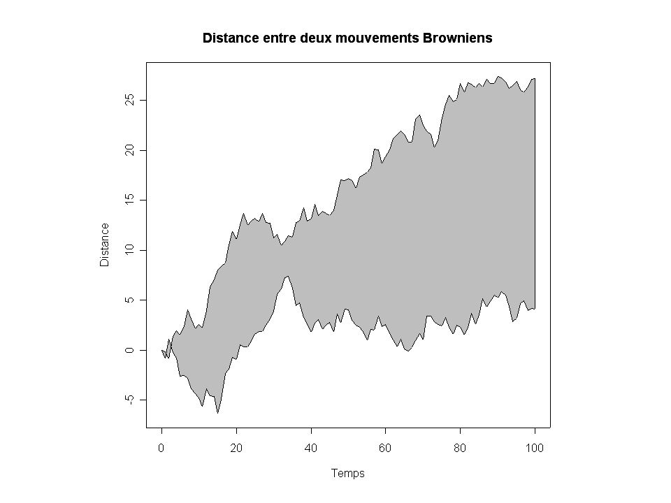
12. par(bg = "white") n = 100 x = c(0, cumsum(rnorm(n))) y = c(0, cumsum(rnorm(n))) xx = c(0:n, n:0) yy = c(x, rev(y)) plot(xx, yy, type = "n", xlab = "Time", ylab = "Distance") polygon(xx, yy, col = "gray") title("Distance entre deux mouvements Browniens")

14. x = c(0, 0.4, 0.86, 0.85, 0.69, 0.48, 0.54, 1.09, 1.11, 1.73, 2.05, 2.02) par(bg = "lightgray"); plot(x, type = "n", axes = FALSE, ann = FALSE); lines(x, col = "blue"); points(x, pch = 21, bg = "lightcyan", cex = 1.25); axis(2, col.axis = "blue", las = 1); axis(1, at = 1:12, lab = month.abb, col.axis = "blue"); box(); title(main = "The Level of Interest in R", font.main = 4, col.main = "red") title(xlab = "1996", col.lab = "red")

15. x=c(…) par(bg = "lightgray"); plot(x, type = "n", axes = FALSE, ann = FALSE);

16. lines(x, col = "blue"); points(x, pch = 21, bg = "lightcyan", cex = 1.25);

17. axis(2, col.axis = "blue", las = 1); axis(1, at = 1:12, lab = month.abb, col.axis = "blue");

18. box(); title(main = "The Level of Interest in R", font.main = 4, col.main = "red") title(xlab = "1996", col.lab = "red")

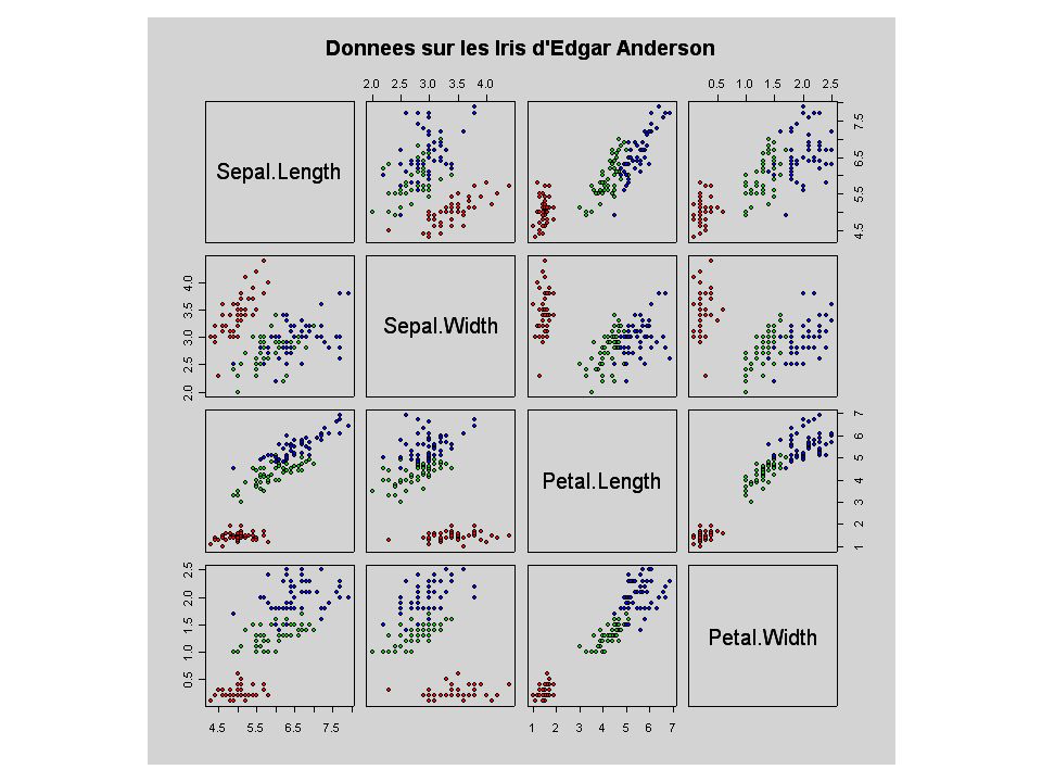
20. La fonction pairs pairs(iris[1:4], main = « donnees sur les Iris d’Edgar Anderson", font.main = 4, pch = 19)

22. La fonction pairs() pairs(iris[1:4], main = « Données sur les Iris d’Edgar Anderson", pch = 21, bg = c("red","green3«,"blue") [unclass(iris$Species)])

24. Résolution de l’ex 1 p40 t=c(2:12);N=c(55,90,135,245,403,66 5,1100,1810,3000,4450,7350) T=data.frame(t,N,y=log(N));T; > T t N y t N y 1 2 55 4.007333 2 3 90 4.499810 3 4 135 4.905275 4 5 245 5.501258…..

25. Calcul de moyenne et écart-type apply(T,2,mean); t N y 7.000000 1754.818182 6.475094 apply(T,2,sd); t N y 3.316625 2326.625317 1.640357

26. plot(T$t,T$N)

27. plot(T$t,T$y)

28. droite de regression ll=lm(y~t,data=T);ll; Call: lm(formula = y ~ t, data = T) Coefficients: (Intercept) t 3.0142 0.4944

29. abline(ll);

30. summary(ll) Call: lm(formula = y ~ t, data = T) Residuals: Min 1Q Median 3Q Max -0.08656 -0.02117 0.01500 0.02912 0.04802 Coefficients: Estimate Std. Error t value Pr(>|t|) (Intercept) 3.014162 0.032947 91.49 1.13e-14 *** t 0.494419 0.004289 115.27 1.41e-15 *** --- Signif. codes: 0 `***' 0.001 `**' 0.01 `*' 0.05 `.' 0.1 ` ' 1

31. summary(ll) suite Residual standard error: 0.04499 on 9 degrees of freedom Multiple R-Squared: 0.9993, Adjusted R- squared: 0.9992 F-statistic: 1.329e+04 on 1 and 9 DF, p-value: 1.413e-15