1. Algorithmic Game Theory and Scheduling Eric Angel, Evripidis Bampis, Fanny Pascual IBISC, University of Evry, France GOTha, 12/05/06, LIP 6

2. Outline  Scheduling vs. Game Theory  Stability, Nash Equilibrium  Price of Anarchy  Coordination Mechanisms  Truthfulness

3. Scheduling (A set of tasks) + (a set of machines) (an objective function) Aim: Find a feasible schedule optimizing the objective function.

4. Game Theory (A set of agents) + (a set of strategies) (an individual obj. function for every agent) Aim: Stability, i.e. a situation where no agent has incentive to unilaterally change strategy. Central notion: Nash Equilibrium (pure or mixed)

5. Game Theory (2) Nash: For any finite game, there is always a (mixed) Nash Equilibrium. Open problem: Is it possible to compute a Nash Equilibrium in polynomial time, even for the case of games with only two agents ?

6. Scheduling & Game Theory The KP model: (Agents: tasks) + (Ind. Obj. F. of agent i: the completion time of the machine on which task i is executed) The CKN model: (Agents: tasks) + (Ind. Obj. F. of agent i: the completion time of task i)

7. Scheduling & Game Theory (2) The AT model: (Agents: uniform machines) + (Ind. Obj. F. of agent i: the profit defined as P i -w i /s i ) P i : payment given to i W i : load of machine i S i : the speed of machine i

8. The Price of Anarchy (PA) Aim: Evaluate the quality of a Nash Equilibrium. [Koutsoupias, Papadimitriou: STACS’99] Need of a Global Objective Function (GOF) PA=(The value of the GOF in the worst NE)/(OPT) It measures the impact of the absence of coordination [In what follows, GOF: makespan]

9. An example: KP model [Koutsoupias, Papadimitriou: STACS’99] 2 1 3 12 13 time 0123 3 tasks 2 machines A (pure) Nash Equilibrium Question: How bad can be a Nash Equilibrium ?

10. An example: KP model pijpij : the probability of task i to go on machine j The expected cost of agent i, if it decides to go on machine j with p i j =1: C i j = l i +  p j k l k K  i In a NE, agent i assigns non zero probabilities only to the machines that minimize C i j

11. An example Instance: 2 tasks of length 1, 2 machines. A NE: p i j = 1/2 for i=1,2 and j=1,2 C 1 1 = 1 + 1/2*1 = 3/2 C 1 2= C 2 1= C 2 2 =3/2 Expected makespan 1/4*2+1/4*2+1/4*1+1/4*1 =3/2 OPT = 1

12. The PA for the KP model Thm [KP99]: The PA is (at least and at most) 3/2 for the KP model with two machines. Thm [CV02]: The PA is  (log m/(log log log m)) for the KP model with m uniform machines.

13. Pure NE for the KP model Thm [FKKMS02]: There is always a pure NE for the KP model. Thm [V02]: The PA (pure Nash eq.), is 2-2/(m+1) for the KP model with m identical machines Thm [CV02]: The PA is  (log m/(log log log m)) for the KP model with m identical machines. Thm [FKKMS02]: It is NP-hard to find the best and worst equilibria.

14. Pure NE for KP and local search Nash eq. => local optimum (with Jump) The converse is not true. 4 4 1 2 5 4 4 1 2 5 A local optimum Not a Nash eq.

15. How can we improve the PA ? Coordination mechanisms Aim: to decrease the PA What kind of mechanisms ? -Local scheduling policies in which the schedule on each machine depends only on the loads of the machine. -each machine can give priorities to the tasks and introduce delays.

16. The LPT-SPT c.m. for the CKN model 11 22 M1 M2 SPT LPT 40 M1 M2 1 1 2 2 3 0 Thm [CKN03]: The LPT-SPT c.m. has a price of anarchy of 4/3 for m=2. [The LPT c.m. has a PA of 4/3-1/3m]

17. The Price of Stability (PS) The framework: A protocol wishes to propose a collective solution to the users that are free to accept it or not. Aim: Find the best (or a near optimal) NE PS = (value of the GOF in the best NE)/OPT Example: - PS=1 for the KP model - PS=4/3-1/3m for the CKN model (with LPT l.p.)

18. Nashification for the KP model Thm [E-DKM03++]: There is a polynomial time algorithm which starting from an arbitrary schedule computes a NE for which the value of the GOF is not greater than the one of the original schedule. Thus: There is a PTAS for computing a NE of minimum social cost for the KP model.

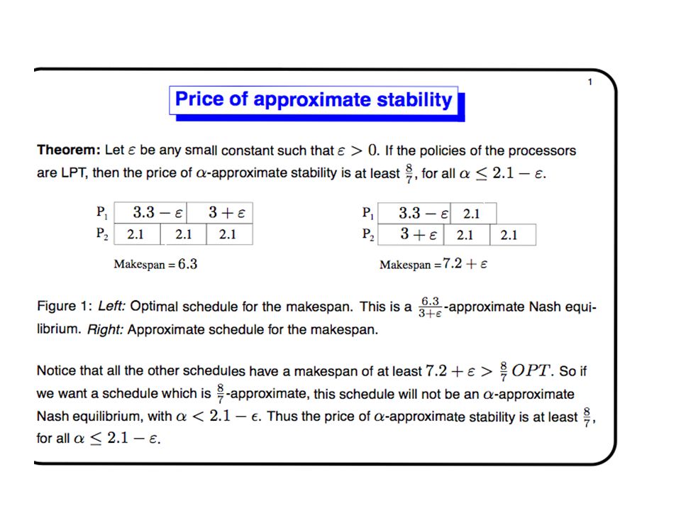
19. Approximate Stability Aim: Relax the notion of stable schedule in order to improve the price of stability.  -approx. NE: a situation in which no agent has sufficient incentive to unilaterally change strategy, i.e. its profit does not increase more than  times its current profit. Example: a 2-approx. NE 33 222 M1 M2 LPT

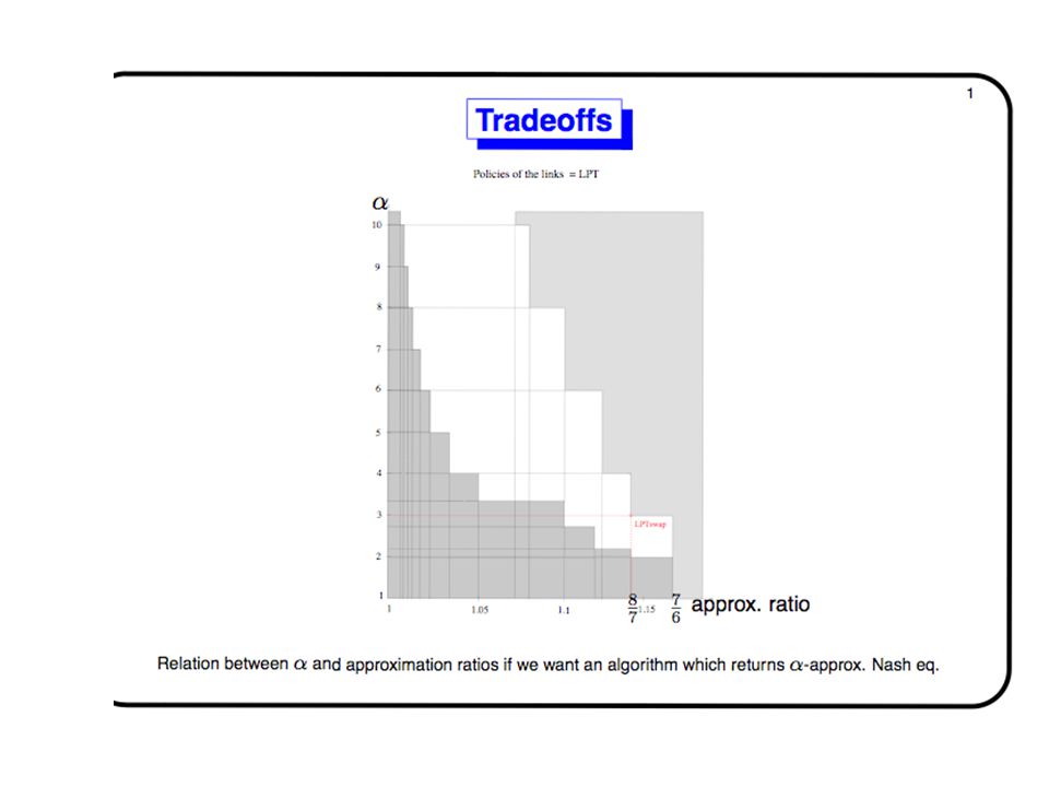
20. The algorithm LPT swap -construct an LPT schedule -1st case: -2nd case: x1x2x3 y1y2 Exchange: (x1,y1), or (x1,y2), or (x2,y2) Return the best or LPT x1x2x3x4 y1y2 Exchange: (x3+x4,y2) Compare with LPT and return the best -3rd case: Return LPT Thm[ABP05]: LPT swap returns a 3-approx. NE and has an approximation ratio of 8/7. Therefore the price of 3-approximate stability is less than 8/7 (LPT l.p).

24. Truthful algorithms The framework: Even the most efficient algorithm may lead to unreasonable solutions if it is not designed to cope with the selfish behavior of the agents.

25. CKN model: Truthful algorithms The approach: –Task i has a secret real length l i. –Each task bids a value b i ≥ l i. –Each task knows the values bidded by the other tasks, and the algorithm. Each task wish to reduce its completion time. Social cost = maximum completion time (makespan) Aim : An algorithm truthful and which minimizes the makespan. [Christodoulou, Koutsoupias, Nanavati: ICALP’04]

26. Two models Each task wish to reduce its completion time (and may lie if necessarily). 2 models: –Model 1: If i bids b i, its length is l i –Model 2: If i bids b i, its length is b i Example: We have 3 tasks:,, Task 1 bids 2.5 instead of 1:. 123 Model 1: C 1 = 1 Model 2: C 1 = 2.5 time 3 12 0123 4 5 1

27. SPT: a truthful algorithm SPT: Schedules greedily the tasks from the smallest one to the largest one. –Example: –Approx. Ratio = 2 – 1/m [Graham] Are there better truthful algorithms ? 1 2 3

28. LPT LPT: Schedules greedily the tasks from the largest one to the smallest one. –Approx. Ratio = 4/3 – 1/(3m) [Graham] We have 3 tasks:,, Task 1 bids 1 : Task 1 bids 2.5 : 123 Task 1 has incentive to bid 2.5, and LPT is not truthful. C 1 = 3 3 2 1 C 1 = 1 time 3 12 0123 4 5 0123 4 5 1

29. Randomized Algorithm Idea: to combine: –A truthful algorithm –An algorithm not truthful but with a good approx. ratio. Task: wants to minimizes its expected completion time. Our Goal: A truthful randomized algorithm with a good approx. ratio.

30. Outline  Truthful algorithm  SPT-LPT is not truthful  Algorithm: SPT   A truthful algorithm: SPT  -LPT

31. SPT-LPT is not truthful Algorithm SPT-LPT: –The tasks bid their values –With a proba. p, returns an SPT schedule. With a proba. (1-p), returns an LPT schedule. We have 3 tasks :,, –Task 1 bids its true value : 1 –Task 1 bids a false value : 2.5 123 1 2 33 2 1 SPT : LPT : C 1 = p + 3(1-p) = 3 - 2p 1 23 SPT : LPT : 3 1 2 C 1 = 1 1 1

32. Algorithm SPT  SPT  : Schedules tasks 1,2,…,n s.t. l 1 < l 2 < … < l n Task (i+1) starts when 1/m of task i has been executed. Example : (m=3) 0123456789 10 11 12 1 2 3 5 6 7 8 9 4

33. Algorithm SPT  Thm: SPT  is (2-1/m)-approximate. Idea of the proof: (m=3) Idle times : idle_beginning(i) = ∑ (1/3 l j ) idle_middle(i) = 1/3 ( l i-3 + l i-2 + l i-1 ) – l i-3 idle_end(i) = l i+1 – 2/3 l i + idle_end(i+1) j<i 0123456789 10 11 12 1 2 3 5 6 7 8 9 4

34. Algorithm SPT  Thm: SPT  is (2-1/m)-approximate. Idea of the proof: (m=3) 0123456789 10 11 12 1 2 3 5 6 7 8 9 4 Cmax = (∑(idle times) + ∑(li)) / m ∑(idle times) ≤ (m-1) l n and l n ≤ OPT  Cmax ≤ ( 2 – 1/m ) OPT Cmax

35. A truthful algorithm: SPT  -LPT Algorithm SPT  -LPT: –With a proba. m/(m+1), returns SPT . –With a proba. 1/(m+1), returns LPT. The expected approx. ratio of SPT  - LPT is smaller than the one of SPT: e.g. for m=2, ratio(SPT  -LPT) < 1.39, ratio(SPT)=1.5 Thm: SPT  -LPT is truthful.

36. A truthful algorithm: SPT  -LPT Thm: SPT  -LPT is truthful. Idea of the proof: Suppose that task i bids b>l i. It is now larger than tasks 1,…, x, smaller than task x+1. l 1 < … < l i < l i+1 < … < l x < l x+1 < … < l n LPT: decrease of C i (lpt) ≤ (l i+1 + … + l x ) SPT  : increase of C i (spt  ) = 1/m (l i+1 + … + l x ) SPT  -LPT: change = - m/(m+1) C i (spt  ) + 1/(m+1) C i (spt  ) ≥ 0 b <

37. AT model: Truthful algorithms Monotonicity: Increasing the speed of exactly one machine does not make the algorithm decrease the work assigned to that machine. Thm [AT01]: A mechanism M=(A,P) is truthful iff A is monotone.

38. An example The greedy algorithm is not monotone. Instance: 1, , 1, 2-3  for  0<  <1/3 Speeds (s1,s2) M1 M2 (1,1)  1, 2-3   (1,2)  2-3  1,1

39. 3-approx randomized mechanism [AT01] (2+  )-approx mechanism for divisible speeds and integer and bounded speeds [ADPP04] (4+  )-approx mechanism for fixed number of machines [ADPP04] 12-approx mechanism for any number of machines [AS05] Results for the AT model

40. Conclusion Future work: -Links between LS and game theory -Many variants of scheduling problems …