1. Discovery of Structural Variation with Next-Generation Sequencing Alexandre Gillet-Markowska Alexandre.gillet-markowska@upmc.fr Gilles Fischer Team – Biology of Genomes UMR7238 Laboratory of Computational and Quantitative Biology Université Pierre et Marie-Curie, Paris

2. (i)Structural variations (SV) (ii) SV detection technologies (iii) Read pairs: 2 types of Illumina genomic DNA libraries (iv) SV detection using Read pairs (v) Polymorphic SV Structural Variations (SV) outline

3. 1 Yes, the minimal size is arbitrary… 1 Structural Variations (SV)

8. INVERSION (INV)RECIPROCAL TRANSLOCATION (RT) INSERTION (INS) DELETION (DEL) ref SV ref SV Balanced SV Unbalanced SV (CNV) Intrachromosomal SVInterchromosomal SV ref SV ref SV TANDEM DUPLICATION (DUP) Balanced SV versus Unbalanced SV Pictures adapted from Feuk et al., 2006 Nature Reviews Calvin Blackman Bridges, Science

9. Why Discover SV ?  involved in > 30 diseases (Psoriasis, Crohn disease, ASD…)  chromosomal instability detected in the vast majority of cancers  powerful mechanism of adaptation and evolution

10. SV detection technologies

11. Calvin Blackman Bridges, Science Timeline of technologies used to discover SV SV, Structural Variations since 1936 1936 Lejeune, Study of somatic chromosomes from 9 mongoloid children, Hebd Seances Acad Sci 1959 Smith et al, Interstitial deletion of (17)(p11.2p11.2) in nine patients. Am J Med Genet 1986 Comparative cytogenetics

12. Calvin Blackman Bridges, Science 200 et 221 CNV 360 Mb CNVR (12% du génome humain) 1936 Lejeune, Study of somatic chromosomes from 9 mongoloid children, Hebd Seances Acad Sci 1959 Smith et al, Interstitial deletion of (17)(p11.2p11.2) in nine patients. Am J Med Genet 1986 Iafrate, Detection of large-scale variation in the human genome, Nature Sebat, Large-scale copy number polymorphism in the human genome, Science 2004 Redon, Global variation in copy number in the human genome, Nature 2006 Comparative cytogenetics Microarrays Timeline of technologies used to discover SV SV, Structural Variations since 1936

13. Calvin Blackman Bridges, Science 200 et 221 CNV 360 Mb CNVR (12% du génome humain) Microarrays Korbel et al, Paired-end mapping reveals extensive structural variation in the human genome, Science NGS 1936 Lejeune, Study of somatic chromosomes from 9 mongoloid children, Hebd Seances Acad Sci 1959 Smith et al, Interstitial deletion of (17)(p11.2p11.2) in nine patients. Am J Med Genet 1986 Iafrate, Detection of large-scale variation in the human genome, Nature Sebat, Large-scale copy number polymorphism in the human genome, Science 2004 Redon, Global variation in copy number in the human genome, Nature 2006 2007 1000 HGP, A map of human genome variation from population-scale sequencing, Nature 2010 20 000 SV 1 000 SV Comparative cytogenetics Timeline of technologies used to discover SV SV, Structural Variations since 1936

14. ‘Range of usability’ of technologies  Size limit  SV type limit

16. SV detection with NGS data

17. Breakpoints res. SV size range CNV Balanced SV FDR Missing rate >100 bp > Insert Size Yes Variable Quinlan & Hall 2011 Trends in Genetics LI 2011 Nature 1 bp 1 bp–50 kbp Yes >10% >25% 1-10 bp >10 bp Yes No High? 1 bp >1 bp Yes low High? How to detect SV with NGS data ?

18. Read pairs: 2 types of Illumina genomic DNA libraries 1) Illumina Paired-End 2) Illumina Mate-Pair

19. 1) Illumina Paired-End

20. 2) Illumina Mate-Pair

21. Illumina Paired end vs Mate-Pair (MP allows a better genome assembly than PE) MP allows to detect SV that involve repeated elements

22. Illumina Paired end vs Mate-Pair Insert-size distribution of 100,000 read-pairs Insert-size (bp) 5,000 (or much less…)

23. Illumina Paired end vs Mate-Pair

24. SV detection with Read pairs 1)trim the data 2)align data to reference genome 3)remove PCR duplicates 4)SV calling

25. Trim the data First criteria: Chargaff rule

26. Trim the data First criteria : %A = %T and %G = %C on both DNA strands

27. Trim the data Second criteria: nucleotide quality Bcbio-nextgen Btrim CANGS Chipster Clean reads ConDeTri Ea-utils Fastx Flexbar PRINSEQ Reaper SeqTrim Skewer SolexaQA TagCleaner Trimmomatic Trimming tools

28. Align the data to reference genome

29. Remove PCR duplicates samtools rmdup (only intra-molecular duplicates) markduplicates.jar (picard tools) FastUniq … PCR duplicates annotation tools

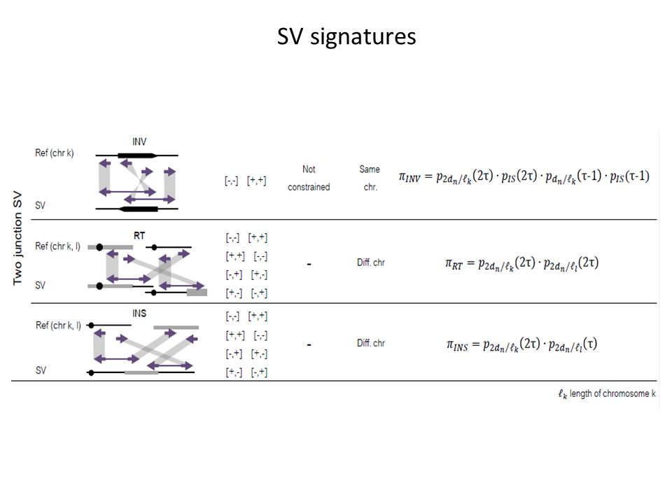
30. SV signatures SV have nearly identical signatures with MP and PE

31. SV signatures Gillet-Markowska, 2014, Bioinformatics

32. SV signatures

34. Inter-tool variability is immense

36. Adapted from ICGC-TCGA challenge

37. Inter-tool variability is immense

38. SV examples

39. Korbel et al, Science 2007 SV in the Human genome

40. Not-so-identical monozygotic twins Bruder, C. E. G. et al. Phenotypically concordant and discordant monozygotic twins display different DNA copy-number-variation profiles. Am. J. Hum. Genet. 82, 763–771 (2008)

41. Butterfly mimicry

43. Livestock phenotypes caused by CNV

44. Polymorphic SV Structural Variations (SV)

45. Individual (germ line) SV in 100% of cells of each individual Tissue (somatic) SV in one tissue / in a few cells Polymorphic SV Structural Variations (SV)

46. #generation Bottleneck 1 60901201502400 Bottleneck 2Bottleneck 3Bottleneck 4Bottleneck 5 Bottleneck 80 030 #cells12410 9 Sequencing a single culture Can we detect de novo SV occurring in a single cell culture by high throughput sequencing ? DNA extraction Sequencing (n=80) DNA extraction Sequencing The physical coverage (theoretically) sets the detection threshold S. cerevisiae 30 # generations 011 10 9 # cells 1 1 2 2 4 12 2.10 3 10 3 13 8.10 3 14 1.6.10 4 6,000X 700X

47. Pair-End sequencing: insert size ~ 400 bp Sequencing with high physical coverage Reference Cell 1 Cell 2 Cell 3 Cell 4 Cell 5 Cell 6 Cell 7 Cell 8 Cell 9 Cell 10

48. Pair-End sequencing: insert size ~ 400 bp Sequencing with high physical coverage Reference Cell 1 Cell 2 Cell 3 Cell 4 Cell 5 Cell 6 Cell 7 Cell 8 Cell 9 Cell 10

49. Pair-End sequencing: insert size ~ 400 bp Sequencing with high physical coverage 2 1 0 Coverage (sequence) cov seq = 0.5X Reference Cell 1 Cell 2 Cell 3 Cell 4 Cell 5 Cell 6 Cell 7 Cell 8 Cell 9 Cell 10

50. Pair-End sequencing: insert size ~ 400 bp Sequencing with high physical coverage 2 1 0 2 1 0 Coverage (sequence) cov seq = 0.5X cov phys = 0.85X Coverage (physical) Reference Cell 1 Cell 2 Cell 3 Cell 4 Cell 5 Cell 6 Cell 7 Cell 8 Cell 9 Cell 10

51. Pair-End sequencing: insert size ~ 400 bp Sequencing with high physical coverage 2 1 0 2 1 0 Coverage (sequence) cov seq = 0.5X cov SV = 0 Reference Cell 1 Cell 2 Cell 3 Cell 4 Cell 5 Cell 6 Cell 7 Cell 8 Cell 9 Cell 10 cov phys = 0.85X Coverage (physical)

52. Mate Pair sequencing: insert size ~ 1 to 20 kb Sequencing with high physical coverage Reference Cell 1 Cell 2 Cell 3 Cell 4 Cell 5 Cell 6 Cell 7 Cell 8 Cell 9 Cell 10 Discordant Paired Sequence

53. Mate Pair sequencing: insert size ~ 1 to 20 kb Sequencing with high physical coverage Reference Cell 1 Cell 2 Cell 3 Cell 4 Cell 5 Cell 6 Cell 7 Cell 8 Cell 9 Cell 10 2 1 0 2 0 4 6 8 10 cov seq = 0.5X cov phys = 5X Coverage (sequence) Coverage (physical) cov SV = 1 Discordant Paired Sequence Mate Pair sequencing increases the sensitivity of SV detection

56. Illumina Paired-End