1. Chaos and the physics of non-equilibrium systems Henk van Beijeren Institute for Theoretical Physics Utrecht University

2. CONTENTS Dynamical systems Lyapunov exponents KS entropy Chaos and approach to equilibrium The Lorentz gas Diffusion coefficient Lyapunov exponents Connections? Collective Lyapunov modes What connections DO exist? Gaussian thermostat formalism Escape rate formalism Hausdorff dimensions of hydrodynamic modes Thermodynamic formalism Other connections Calculations for moving spheres or disks Conclusions

3. Dynamical Systems Theory: For flows:

4. For maps:

5. Lyapunov exponents:

6. Kolmogorov-Sinai entropy

7. Pesin’s theorem:

8. Gibbs assigns approach to equilibrium to mixing and coarse- graining. Is chaos related to approach to equilibrium?

9. The KS entropy describes the average rate of spreading in the expanding directions. Suggests this may be a measure of the speed of mixing and thus of the approach to equilibrium (at least in ergodic systems).

10. Perhaps one should use the smallest positive Lyapunov exponent as a measure for the slowest decay to equilibrium.

11. The KS entropy describes the average rate of spreading in the expanding directions. Suggests this may be a measure of the speed of mixing and thus of the approach to equilibrium (at least in ergodic systems). Perhaps one should use the smallest Lyapunov exponent as a measure for the slowest decay to equilibrium. Can one somehow connect these concepts?

12. Twodimensional Lorentz gas Regular Sinai-billiard

13. Random Lorentz gas

15. There is one positive Lyapunov exponent. It may be estimated easily:

18. Density dependences are very different.

19. Various other differences as well: –Diffusion coefficient diverges for Sinai billiard with infinite horizon.

21. Density dependences are very different. Various other differences as well: –Diffusion coefficient diverges for Sinai billiard with infinite horizon. –Diffusion coefficient vanishes below percolation density.

23. Density dependences are very different. Various other differences as well: –Diffusion coefficient diverges for Sinai billiard with infinite horizon. –Diffusion coefficient vanishes below percolation density. –Wind tree model has diffusive behavior on large time and length scales, but zero Lyapunov exponents.

24. Wind tree model

25. System behaves diffusively on large time and length scales. It shows mixing behavior, but power law with time. So the KS entropy equals zero. Perhaps a definition of weak, nonexponential chaos is needed to describe this. only increases as a

26. Density dependences are very different. Various other differences as well: –Diffusion coefficient diverges for Sinai billiard with infinite horizon. –Diffusion coefficient vanishes below percolation density. –Wind tree model has diffusive behavior on large time and length scales, but zero Lyapunov exponents. No obvious connections between Lyapunov exponent and hydrodynamic decay!

27. Are smallest Lyapunov exponents of many- particle systems related to hydrodynamics? Lyapunov spectrum for 750 hard disks (Posch and coworkers)

28. Like in hydrodynamics there are branches of k-dependent eigenvalues that approach zero in the limit In the limitboth sets of eigenvalues approach zero, because the corresponding eigenmodes appoach to a symmetry transformation. But no connection between the eigenvalues appears. Lyapunov “shear” mode. Average velocity deviation in x-direction as a function of y-coordinate. Growth rate is proportional to k (vs. decay rate ~ k 2 for hydrodynamic shear mode).

29. What connections do exist?

30. Most of them consider changes in dynamical properties due to deviations from equilibrium. 1. Gaussian thermostat formalism of Evans and Hoover:

31. Systems under external driving forces are kept at constant kinetic (or total) energy by applying fictitious thermostat forces, such that Here has to be chosen such that the kinetic energy (or the total energy) remains strictly constant. For such and a few different fictitious thermostats, minus the sum of all Lyapunov exponents (the average rate of phase space contraction!) can be identified with the rate of irreversible entropy production.

32. What connections do exist? Most of them consider changes in dynamical properties due to deviations from equilibrium. 1.Gaussian thermostat formalism of Evans and Hoover: 2.The escape rate formalism of Gaspard and Nicolis.

33. For finite systems with open boundaries, through which trajectories may escape, the KS entropy satisfies For diffusive systems connects a transport coefficient with dynamical systems properties. so this relationship Survival rate of

34. What connections do exist? Most of them consider changes in dynamical properties due to deviations from equilibrium. 1.Gaussian thermostat formalism of Evans and Hoover: 2.The escape rate formalism of Gaspard and Nicolis. 3.Relationships between Hausdorff dimensions of hydrodynamic modes, Lyapunov exponents and transport coefficients, obtained by Gaspard et al.

35. For two-dimensional diffusive systems, Gaspard, Claus, Gilbert and Dorfman obtained the relationship This can probably be generalized to higher dimensions and general classes of transport coefficients.

36. Other connections between dynamical systems theory and nonequilibrium statistical mechanics involve: 1.Fluctuation theorems (Evans, Morriss, Searles, Cohen, Gallavotti and others) relate the probabilities of finding fluctuations in stationary systems with entropy changes of respectively

37. Other connections between dynamical systems theory and nonequilibrium statistical mechanics involve: 1.Fluctuation theorems (Evans, Morriss, Searles, Cohen, Gallavotti, Kurchan, Lebowitz, Spohn and others) relate the probabilities of finding fluctuations in stationary systems with entropy changes of respectively 2. Work theorems (Jarzynski and others) allow calculations of free energy differences between different equilibrium states from work done in nonequilibrium processes.

38. Other connections between dynamical systems theory and nonequilibrium statistical mechanics involve: 1.Fluctuation theorems (Evans, Morriss, Searles, Cohen, Gallavotti, Kurchan, Lebowitz, Spohn and others) relate the probabilities of finding fluctuations in stationary systems with entropy changes of respectively 2. Work theorems (Jarzynski and others) allow calculations of free energy differences between different equilibrium states from work done in nonequilibrium processes. 3. Ruelle’s thermodynamic formalism.

39. Dynamical partition function: Topological pressure: In general,

40. 4. SRB (Sinai-Ruelle-Bowen) measures may provide a general tool for describing stationary nonequilibrium states. These are the stationary distributions to which arbitrary initial distributions approach asymptotically. For ergodic Hamiltonian systems they coincide with the microcanonical distribution, for phase space contracting systems they are smooth in the expanding directions and have a highly fractal structure in the contracting directions.

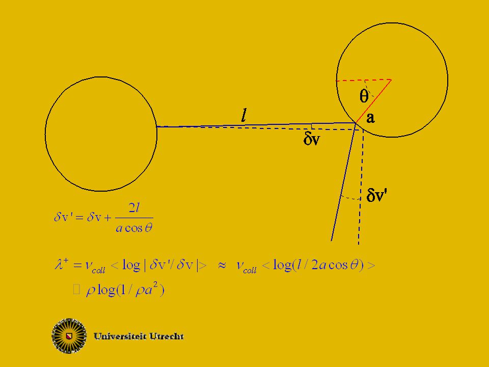
41. For moving hard speres at low density the velocity deviations of two colliding particles are both upgraded to a value of the order of. Moving hard spheres and disks

42. Set The distribution of these “clock values” approximately satisfies:. Can be solved for stationary profile of the form P(n,t)=P(n-vt) by linearizing for large n. Then v log(l mf /a) is the largest Lyapunov exponent. It is determined by.

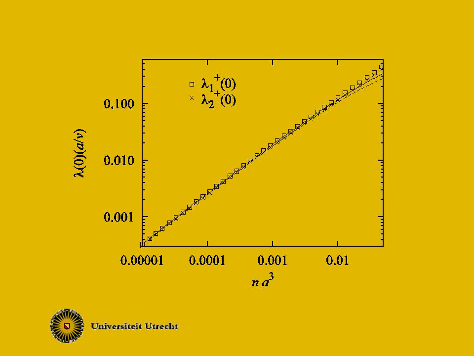
43. Gives rise to largest Lyapunov exponent Keeping account of velocity dependence of collision frequency one may refine this to Finite size corrections are found to behave as May be compared to simulation results:

45. Brownian motion We consider a large sphere or disk of radius A and mass M in a dilute bath of disks/spheres of radius a and mass m. At collisions, the velocity deviations of the small particles change much more strongly than those of the Brownian particle. But, because the collision frequency of the latter is much higher, it may still dominate the largest Lyapunov exponent. The process may be characterized by a stationary distribution of the variables can be identified as the largest Lyapunov exponent connected to the Brownian particle.

46. These satisfy the Fokker-Planck equation, Both “diffusion constants” are proportional to Therefore scales as

48. Maximal Lyapunov exponent for 2d system with 40 disks of a=1/2 and m=1. Open squares: pure_fluid. Crosses: A=5 and M=100. Closed squares: A=1/(2√n).

49. Conclusions: There are several connections between dynamical systems theory and nonequilibrium statistical mechanics,but none of them is particularly simple. Dynamical properties of equilibrium systems seem unrelated to traditional properties of decay to equilibrium. Fluctuation and work theorems look potentially useful. SRB-measures may be the tool to use in stationary nonequilibrium states.

50. Thanks to many collaborators: Bob Dorfman Ramses van Zon Astrid de Wijn Oliver Mülken Harald Posch Christoph Dellago Arnulf Latz Debabrata Panja Eddie Cohen Carl Dettmann Pierre Gaspard Isabelle Claus Cécile Appert Matthieu Ernst