Download presentation
Presentation is loading. Please wait.

1
Status and performance of HIRLAM 4D-Var Nils Gustafsson

2
Who made the HIRLAM 4D-Var? Nils Gustafsson Hans Xiang-Yu Huang Xiaohua Yang Magnus Lindskog Kristian Mogensen Ole Vignes Tomas Wilhelmsson Sigurdur Thorsteinsson

3
HIRLAM 4D-Var Developments. 1995-1997: Tangent linear and adjoint of the Eulerian spectral adiabatic HIRLAM. Sensitivity experiments. 1997-1998: Tangent linear and adjoints of the full HIRLAM physics. 2000: First experiments with ”non-incremental” 4D-Var. 2001-2002: Incremental 4D-Var. Simplified physics packages (Buizza vertical diffusion and Meteo France package). 2002: 4D-Var feasibility study. 2003:Semi-Lagrangian scheme (SETTLS), outer loops (spectral or gridpoint HIRLAM) and multi-incremental minimization. 2005: Reference system scripts. Extensive tests of 4D-Var 2006: Continued extensive tests. Weak digital filter constraint. Control of lateral boundary conditions
. 2002: 4D-Var feasibility study. 2003:Semi-Lagrangian scheme (SETTLS), outer loops (spectral or gridpoint HIRLAM) and multi-incremental minimization. 2005: Reference system scripts. Extensive tests of 4D-Var 2006: Continued extensive tests. Weak digital filter constraint. Control of lateral boundary conditions.")
4
Multi-incremental minimization with N τ steps in an outer loop For each step in the outer loop, the TL/AD models and the observation operators are re-linearized around a non-linear full resolution model solution and a quadratic minimization problem is solved.

5
Semi-implicit semi-Lagrangian scheme for the HIRLAM 4D-Var (SETTLS, Hortal)
")
6
Status of HIRLAM 4D-Var TL and AD physics TL and AD versions of the HIRLAM physics were originally derived. These turned out to be very expensive due to many mutual dependencies between processes. The “Buizza” simplified physics is available (vertical diffusion of momentum + surface friction). The simplified Meteo France physics package (Janiskova) is available. Vertical diffusion and large-scale condensation have been used in most HIRLAM 4D-Var tests. The large-scale condensation sometimes contributes to instabilities and minimization divergence at “high” horizontal resolution of increments (40 km).
. The simplified Meteo France physics package (Janiskova) is available. Vertical diffusion and large-scale condensation have been used in most HIRLAM 4D-Var tests. The large-scale condensation sometimes contributes to instabilities and minimization divergence at high horizontal resolution of increments (40 km)..")
7
Single observation experiment with HIRLAM 4D-Var; What is the effect of a single surface pressure observation increment of -5 hPa at + 5 hours in the assimilation window? 1 1: In the center of a developing low 2 2. In a less dynamically active area

8
Surface pressure increments for the Danish storm 3D-Var 4D-Var, spectral TL prop. of incr 4D-Var; gp model prop. of incr.

9
Effects of a -5 hPa surface pressure observation increment at +5 h on the initial wind and temperature increments Winds at model level 20 (500 hPa) and temperatures at level 30 (below) NW-SE cross section with temperatures and normal winds
 and temperatures at level 30 (below) NW-SE cross section with temperatures and normal winds")
10
Effects of a -5 hPa surface pressure observation increment at +5 h in a less dynamically active area Surface pressure assimilation increment at +0 h Difference between non-linear forecasts at +6 h with and without the 4D-Var assimilation increment

11
Recent 4D-Var tests The SMHI 22 km area (306x306x40 gridpoints) SMHI operational observations (including AMSU-A and ”extra” AMDAR observations) 6 h assimilation cycle; 3D-Var with FGAT; 6 h assimilation window in 4D-Var; 1 h observation windows 66 km assimilation increments in 4D-Var (linear grid); 44 km assimilation increments in 3D-Var (quadratic grid) Statistical balance structure functions (the NMC method) Meteo-France simplified physics (VDIFF+LSC) Non-linear propagation of assimilation increments 3 months of data (January 2005, June 2005, January 2006)
 SMHI operational observations (including AMSU-A and extra AMDAR observations) 6 h assimilation cycle; 3D-Var with FGAT; 6 h assimilation window in 4D-Var; 1 h observation windows 66 km assimilation increments in 4D-Var (linear grid); 44 km assimilation increments in 3D-Var (quadratic grid) Statistical balance structure functions (the NMC method) Meteo-France simplified physics (VDIFF+LSC) Non-linear propagation of assimilation increments 3 months of data (January 2005, June 2005, January 2006)")
12
Average upper air forecast verification scores – January 2005 o3d = 3D-Var o4d = 4D-Var Wind speedTemperature

13
Average upper air forecast verification scores – January 2006 o3d = 3D-Var o4d = 4D-Var Wind speed Temperature

14
Mean sea level pressure forecast verification scores – January 2005 o3d = 3D-Var o4d = 4D-Var

15
Mean sea level pressure forecast verification scores – January 2006 o3d = 3D-Var o4d = 4D-Var

16
Time series of mean sea level pressure verification scores – January 2005 o3d = 3dvar o4d = 4D-Var

17
Time series of mean sea level pressure verification scores – January 2006 o3d = 3dvar o4d = 4D-Var

18
Gudrun +48 h with 4D-Var and 3D-Var 3D-Var +0 h 3D-Var +48 h 4D-Var +0 h 4D-Var +48 h

19
12 January 2005 case 3D-Var +0 h 4D-Var +0 h 3D-Var +36 h 4D-Var +36 h

20
25 January 2006 case 3D-Var +0 h 4D-Var +0 h 3D-Var +24 h 4D-Var +24 h

21
Does 4D-Var smooth too much??

22
Computer timings SMHI LINUX-cluster DUNDER – Dual Intel Xeon 3,4 GHz, 2Gb mem/node, Infiniband interconnect 13 nodes (26 proc) were used Average example (3 Jan 2006 12UTC) 48 h forecast (22 km): 1005 seconds 66 km resolution 4D-Var : 1053 seconds 82 iterations (88 simulations) 30 min timestep 44 km resolution 4D-Var : 3971 seconds 90 iterations (97 simulations) 15 min timestep
 were used Average example (3 Jan UTC) 48 h forecast (22 km): 1005 seconds 66 km resolution 4D-Var : 1053 seconds 82 iterations (88 simulations) 30 min timestep 44 km resolution 4D-Var : 3971 seconds 90 iterations (97 simulations) 15 min timestep")
23
Weak digital filter constraint

24
Reduction of noise (spectral model)
")
25
Noise in assimilation cycles with the gridpoint model

26
Spinup of clouds 3D- Var

27
Spinup of clouds 4D- Var

28
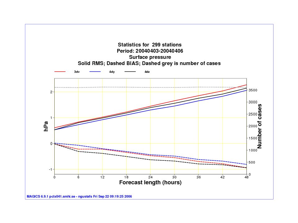
3 4D-Var runs for April 2004 4dv: NMI constraint, non-linear prop. of increments 4dx: J_c_dfi, non-linear prop. of increments 4dy: J_c_dfi, tangent-linear prop. of increments

29
Best 4D-Var run against 3D-Var

30
Control of Lateral Boundary Conditions (1) Introduce the LBCs at the end of the data assimilation window as assimilation control variables (full model state = double size control vector) (2) Introduce the adjoints of the Davies LBC relaxation scheme and the time interpolation of the LBCs (3) Introduce a “smoothing and balancing” constraint for the LBCs into the cost function to be minimized J = J b + J o + J c + J lbc where J lbc = (X lbc - (X lbc ) b ) T B -1 (X lbc - (X lbc ) b ) and B is identical to B for the background constraint
 Introduce the LBCs at the end of the data assimilation window as assimilation control variables (full model state = double size control vector) (2) Introduce the adjoints of the Davies LBC relaxation scheme and the time interpolation of the LBCs (3) Introduce a smoothing and balancing constraint for the LBCs into the cost function to be minimized J = J b + J o + J c + J lbc where J lbc = (X lbc - (X lbc ) b ) T B -1 (X lbc - (X lbc ) b ) and B is identical to B for the background constraint")
31
Example, first cycle with lbc control 21 UTC, start of window 00 UTC Nominal analysis time

32
+12 h +24 h

33
+48 h

35
Problems with Control of LBC 2* control vector Pre-conditioning; LBC_0h and LBC_6h are correlated; (LBC_6h-LBC_0h instead?) Relative weights for J_b and J_lbc??
 Relative weights for J_b and J_lbc")
36
Tangent-Linear Physics Non-linear model with full HIRLAM physics Adiabatic tangent-linear model Buizza vertical diffusion in tangent-linear model (Buizza, ECMWF Tech. Mem. 192, 1993) MF1. Météo-France vertical diffusion in tangent- linear model (Janiskova et al., MWR, 1999) MF2. Météo-France vertical diffusion and large scale condensation in tangent-linear model (Janiskova et al., MWR, 1999) (Météo-France tangent-linear radiation, convection,gravity wave drag are not applied)
 MF1. Météo-France vertical diffusion in tangent- linear model (Janiskova et al., MWR, 1999) MF2. Météo-France vertical diffusion and large scale condensation in tangent-linear model (Janiskova et al., MWR, 1999) (Météo-France tangent-linear radiation, convection,gravity wave drag are not applied).")
37
Cross-section 2005062318 Rel.hum. (MF2), spec hum diff. (MF2-MF1) Rel.hum. (MF1), spec hum diff. (MF2-MF1)
 Rel.hum. (MF1), spec hum diff. (MF2-MF1).")
38
Current urgent problems to be solved : Difficult to show the same positive impact on the ECMWF IBM computer as on the SMHI LINUX-cluster! Convergence of the minimization for some cases

39
Concluding remarks HIRLAM 4D-Var is prepared for near real time tests. Can we afford it operationally? Yes! 4D-Var provide significantly improved forecast scores compared to 3D-Var for synoptic scales and “dynamical” forecast variables (SMHI area and computer only?). Some minimization convergence problems need to be solved. We need to look further into the handling of moist processes.
. Some minimization convergence problems need to be solved. We need to look further into the handling of moist processes..")
40
Future issues Optimized 4D-Var for a 10 km model Improved simplified TL and AD physics Extended use of remote sensing data (radar winds, ground-based GPS, SEVIRI clear and cloudy radiances) Short time window 4D-Var for nowcasting purposes ALADIN 4D-Var for the mesoscale?
 Short time window 4D-Var for nowcasting purposes ALADIN 4D-Var for the mesoscale")
Similar presentations


 (James Hamilton -- Met Éireann)>")


